Chapter 8 ANOVA
Supplement to chapter 5 of Ramsey and Schafer’s Statistical Sleuth 3ED for POL90: Statistics.
knitr::opts_chunk$set(echo = TRUE)8.1 Diet and Longevity
Does restricting calorie intake dramatically increase life expectancy? Researchers randomly assigned 349 female rats to one of six groups, with slight dietary modifications.
We begin by loading packages, reading in and visualizing the data.
# Loading required packages
library(Sleuth3)
library(janitor)
##
## Attaching package: 'janitor'## The following objects are masked from 'package:stats':
##
## chisq.test, fisher.testsuppressMessages(library(dplyr))
library(ggplot2)
library(xtable)# Loading and cleaning dataset
mice <- Sleuth3::case0501 %>% clean_names()
# Viewing dataset and summary
head(mice, 2)## lifetime diet
## 1 35.5 NP
## 2 35.4 NP# Plotting data on diet
ggplot(data=mice) +
aes(x = diet, y = lifetime) +
geom_boxplot() +
ggtitle("Boxplot of lifetimes by diet")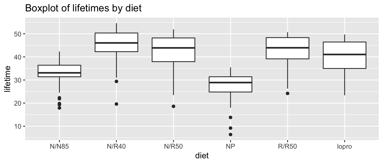
# Plotting data on lifetime
ggplot(data = mice) +
  aes(x = lifetime, color = diet) +
  geom_density() +
  scale_x_continuous(limit = c(0,60)) +
  ggtitle("Density plot of lifetimes by diet")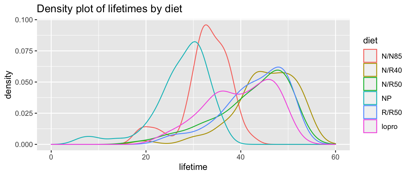
At this point, we want to know whether these groups of mice are significantly different or not. More precisely, we ask whether the means of these specific groups are distinct, or if these observed differences can be explained by random experimental quirk. To answer this question, we use the Analysis of Variance (ANOVA) test.
8.1.1 Analysis of Variance (ANOVA) test
The ANOVA test proposes the null hypothesis that the means of all groups are the same. And thus the alternative hypothesis is that not all means are the same.
In the case of diets and longevity of mice, we have six groups. And so the null hypothesis is that:
\[ \mu_1 = \mu_2 = \mu_3 = \mu_4 = \mu_5 = \mu_6 \]
And the alternative hypothesis is that at least one equality does not hold.
To test this hypothesis, we use the Extra Sum of Squares Principle.
First, we establish the two models: the reduced, or equal-means model, and the full, or separate-means model. Note it is called “reduced” because we impose a restriction of the null hypothesis on the group means.
| Group | 1 | 2 | 3 | 4 | 5 | 6 |
|---|---|---|---|---|---|---|
| Full/Separate-Means Model | \(\overline{Y}_1\) | \(\overline{Y}_2\) | \(\overline{Y}_3\) | \(\overline{Y}_4\) | \(\overline{Y}_5\) | \(\overline{Y}_6\) |
| Reduced/Equal-Means Model | \(\overline{Y}\) | \(\overline{Y}\) | \(\overline{Y}\) | \(\overline{Y}\) | \(\overline{Y}\) | \(\overline{Y}\) |
Table 1: Full and Reduced Models
Now each individual mouse, we observe an observation \(Y_{i,j}\) where \(i\) is the dietary group of the mouse, and \(j\) is the mouse itself.
For each observation, we calculate the residuals in each of the Separate-Means (\(Y_{i,j} - \overline{Y_i}\)) and Equal-Means models (\(Y_{i,j} - \overline{Y}\)). The magnitudes of residual from the equal-means model tends to be larger.
We then calculate the Residual Sum of Squares (or the Sum of Squared Residuals) for each of the models, and then we calculate the Extra Sum of Squares.
\[ \text{Extra Sum of Squares} = \text{Residual sum of squares (reduced)} - \text{Residual sum of squares (full)} \]
A residual sum of squares captures the amount of variation in the observations that cannot be explained by the model. And so, the Extra Sum of Squares measures the amount of variation in the reduced model that is explained by the full model.
We then use this Extra Sum of Squares to determine the plausibility of the null hypothesis by calculating an \(F\)-Statistic.
\[ F-Statistic = \frac{(\text{Extra Sum of Squares})/(\text{Extra Degrees of Freedom})}{\sigma_{full}^2} \]
where the “extra degrees of freedom” is the number of parameters in the mean for the full model (Here: six) minus the number of parameters in the mean for the reduced model (here: one).
An \(F\)-statistic between 0.5 and 3 is considered typical. Between 3 and 4 is considered highly unlikely, and an \(F\)-statistic of greater than 4 suggests that it is extremely unlikely that the means are the same.
The anova() function in R allows us carry out the analytical procedure.
anova_mice <- lm(lifetime ~ diet, data = mice) %>% anova()
anova_mice
## Analysis of Variance Table
##
## Response: lifetime
## Df Sum Sq Mean Sq F value Pr(>F)
## diet 5 12734 2546.8 57.104 < 2.2e-16 ***
## Residuals 343 15297 44.6
## ---
## Signif. codes: 0 '***' 0.001 '**' 0.01 '*' 0.05 '.' 0.1 ' ' 1Tip: the xtable() library and function allows us to render tables in Latex and html.
# Loading xtable
library(xtable)

# Printing table with xtable
anova_mice %>%
  xtable() %>%
print(type = "html")| Df | Sum Sq | Mean Sq | F value | Pr(>F) | |
|---|---|---|---|---|---|
| diet | 5 | 12733.94 | 2546.79 | 57.10 | 0.0000 |
| Residuals | 343 | 15297.42 | 44.60 |
We can also use kableExtra to create tables.
# Loading required packages
library(kableExtra)
##
## Attaching package: 'kableExtra'## The following object is masked from 'package:dplyr':
##
## group_rows# Printing options for tables using kable
options(knitr.kable.NA = "", digits = 4)
anova_mice %>%
kable() %>%
kable_styling()| Df | Sum Sq | Mean Sq | F value | Pr(>F) | |
|---|---|---|---|---|---|
| diet | 5 | 12734 | 2546.8 | 57.1 | 0 |
| Residuals | 343 | 15297 | 44.6 |
And so, with an \(F\)-value of 51.70, and a p-value approximately zero, we can confidently reject the null hypothesis that the means between all six dietary groups is the same.
We use the linear model (regression, called by the lm() function) to do a pairwise comparison of each group, by default, compared to the first group. A summary of the linear model would explicate this comparison more clearly.
lm_out <- lm(lifetime ~ diet, data = mice)
summary(lm_out)
##
## Call:
## lm(formula = lifetime ~ diet, data = mice)
##
## Residuals:
## Min 1Q Median 3Q Max
## -25.517 -3.386 0.814 5.183 10.014
##
## Coefficients:
## Estimate Std. Error t value Pr(>|t|)
## (Intercept) 32.691 0.885 36.96 < 2e-16 ***
## dietN/R40 12.425 1.235 10.06 < 2e-16 ***
## dietN/R50 9.606 1.188 8.09 1.1e-14 ***
## dietNP -5.289 1.301 -4.07 5.9e-05 ***
## dietR/R50 10.194 1.257 8.11 8.9e-15 ***
## dietlopro 6.994 1.257 5.57 5.2e-08 ***
## ---
## Signif. codes: 0 '***' 0.001 '**' 0.01 '*' 0.05 '.' 0.1 ' ' 1
##
## Residual standard error: 6.68 on 343 degrees of freedom
## Multiple R-squared: 0.454, Adjusted R-squared: 0.446
## F-statistic: 57.1 on 5 and 343 DF, p-value: <2e-16Here, the reference group is N/N85, and then as we move from the reference group to the other groups (e.g. N/R40), we see the estimated associated change in mean of lifetime (e.g. increase by 12.4254 units, with p-value close to zero).
Instead, if we are interested in comparing the effects of moving from one specific group to another (rather than including all groups), we can subset the data and run an ANOVA test again.
For example, if we are interested in finding the effect of longevity between the standard diet (NP) and mild caloric intake (N/N85), we could use the following procedure:
# note: vertical line | is the logical operator "OR".
mice_np_vs_nn85 <- mice %>%
  filter(diet == "NP" | diet == "N/N85")

anova_mice_np_nn85 <- lm(lifetime ~ diet, data = mice_np_vs_nn85) %>% anova()
anova_mice_np_nn85 %>%
xtable() %>%
print(type = "html")| Df | Sum Sq | Mean Sq | F value | Pr(>F) | |
|---|---|---|---|---|---|
| diet | 1 | 737.13 | 737.13 | 23.39 | 0.0000 |
| Residuals | 104 | 3276.92 | 31.51 |
With an \(F\)-value of close to 24, and a p-value approximately zero, we can reject the null hypothesis that the mean of longevity between the two dietary groups are the same.
We can perform the same procedure for any combination of groups.
8.2 Developing an intuition for ANOVA using infer
We can use the infer package, which you encountered earlier, to develop an intuition for ANOVA in general, and the \(F\)-Statistic in particular. Remember that we want to know whether the values we observe as mean outcomes for each treatment group are significantly different from each other, or whether they can be explain as just random variations. One way to think of this is to imagine that we randomly reassigned our observed values from each treatment (like the randomization tests of Chapter 1), and then calculated the mean by group. How extreme would the \(F\)-statistic associated with the means we originally observed be, as compared to that of each of the group means we now have?
infer allows us to do this. By calculating the \(F\)-statistic of all the new permutations we create, we can identify how unique our \(F\)-statistic is. We will first specify what our treatment result variable and our explanatory variable, which will be categorical, are. We will then hypothesize our null, which is that there is no relationship between these two variables, i.e., they are independent. The next step will be to generate a number of permutations, where our results will be reassigned to different treatment conditions. We will finally calculate the \(F\)-statistic for each of these permutations.
library(infer)

mice_permutations <- mice %>%
  filter(diet == "NP" | diet == "N/R50" | diet == "N/N85") %>%

  specify(lifetime ~ diet) %>%
  hypothesize(null = "independence") %>%
  generate(reps = 1000, type = "permute") %>%
  calculate(stat = "F")
## Dropping unused factor levels c("N/R40", "R/R50", "lopro") from the supplied explanatory variable 'diet'.head(mice_permutations)## Response: lifetime (numeric)
## Explanatory: diet (factor)
## Null Hypothesis: independence
## # A tibble: 6 × 2
## replicate stat
## <int> <dbl>
## 1 1 2.39
## 2 2 0.688
## 3 3 0.343
## 4 4 1.02
## 5 5 0.291
## 6 6 0.342With infer we could plot a histogram using visualize(mice_permutations) that creates a ggplot histogram. We can also easily create the histogram from scratch and add where our observed \(F\)-statistic falls on this plot. Our \(F\)-statistic is an element in the output produced by our NP vs N/N85 anova call, anova_mice_np_nn85.
anova_mice_np_nn85_fstat <- anova_mice_np_nn85$`F value`

ggplot(mice_permutations) +
  aes(x = stat) +
  geom_histogram() +
  geom_vline(xintercept = anova_mice_np_nn85_fstat,
             col = "red")
## `stat_bin()` using `bins = 30`. Pick better value with `binwidth`.## Warning: Removed 1 rows containing missing values (geom_vline).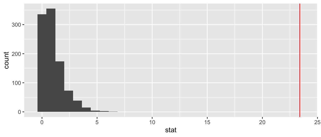
Our observed value is extreme relative to the distribution, giving us a fair degree of confidence that the variation in our observed means is not likely to be due to a statistical fluke. The differences are statistically significant.
8.3 Spock Conspiracy Trial
In 1968, Dr Benjamin Spock was put on trial for conspiring to violate the Selective Services Act by encouraging young men to resist the draft for the Vietnam war. Dr Spock’s defense challenged the method by which jurors were selected, specifically pointing to the under-representation of women in the jury.
Were women actually underrepresented in his jury pool (or venire)?
We begin by reading in and summarizing the data.
# Reading data
spock <- Sleuth3::case0502 %>% clean_names()

# Viewing first two rows of dataset
head(spock, 2)
## percent judge
## 1 6.4 Spock's
## 2 8.7 Spock's# Viewing percentage summaries for each judge
spock %>%
group_by(judge) %>%
summarize(judge_mean = mean(percent))## # A tibble: 7 × 2
## judge judge_mean
## <fct> <dbl>
## 1 A 34.1
## 2 B 33.6
## 3 C 29.1
## 4 D 27
## 5 E 27.0
## 6 F 26.8
## 7 Spock's 14.6# Viewing data using ggplot
ggplot(data=spock) +
aes(x = judge, y = percent) +
geom_boxplot() +
ggtitle("Boxplot of percentage of women in venire by judge")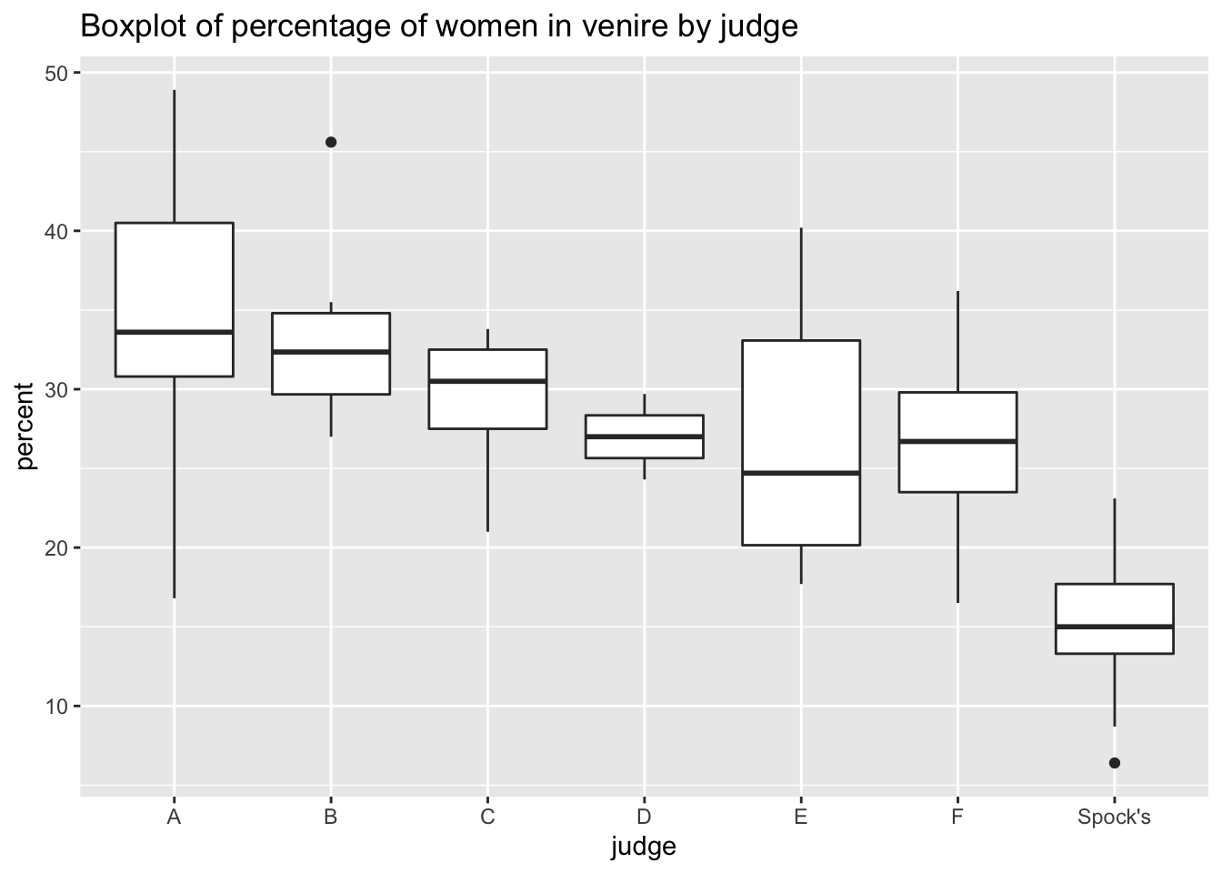
ggplot(data = spock) +
  aes(x = percent, color = judge) +
  geom_density() +
  scale_x_continuous(limit = c(0,60)) +
  ggtitle("Density plot of percent of women in venire by judge")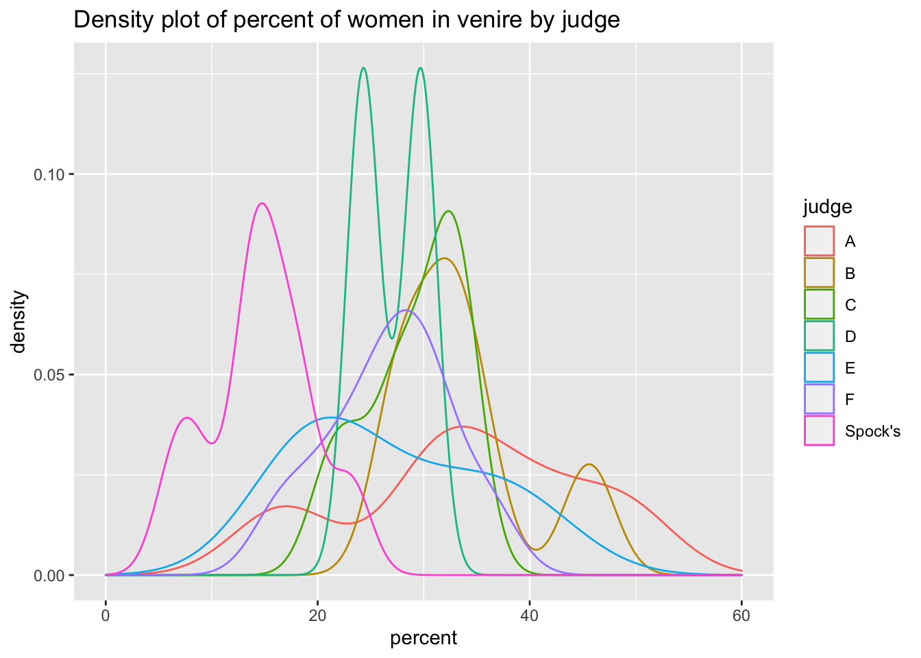
At first glance, it seems like Dr Spock’s judge seems to systematically include fewer women in his venire than other judges.
At this time, we can apply an ANOVA test to test whether the means between groups are actually the same or not.
# Running anova
anova_spock_all <- lm(percent ~ judge, data = spock) %>% anova()
# Printing results using xtable
anova_spock_all %>%
xtable() %>%
print(type = "html")| Df | Sum Sq | Mean Sq | F value | Pr(>F) | |
|---|---|---|---|---|---|
| judge | 6 | 1927.08 | 321.18 | 6.72 | 0.0001 |
| Residuals | 39 | 1864.45 | 47.81 |
With an \(F\)-value greater than 4, we can have great confidence in rejecting the null hypothesis that all means are the same across judges.
The more interesting question for us, however, would be to ask if Spock’s judge, specifically, has significantly fewer women in his venire than all other judges.
We begin by asking if all other judges have approximately the same percentage of women in their venires. For this, we simply subset the data by removing Spock’s judge.
all_but_spock <- spock %>%
  dplyr::filter(judge != "Spock's")

all_but_spock <- lm(percent ~ judge, data = all_but_spock) %>% anova()
all_but_spock %>%
xtable() %>%
print(type = "html")| Df | Sum Sq | Mean Sq | F value | Pr(>F) | |
|---|---|---|---|---|---|
| judge | 5 | 326.46 | 65.29 | 1.22 | 0.3239 |
| Residuals | 31 | 1661.33 | 53.59 |
With an \(F\)-value of 1.22, we cannot reject the null hypothesis that the means between judges A through F are the same.
To compare Spock’s judge to all the other judges, we create a variable that classifies judges as either Spock’s or Not Spock’s, and then conduct the same test.
spock <- spock %>%
  mutate(two_judge = judge != "Spock's") # create a binary for spock / not spock

spock_two_group <- lm(percent ~ two_judge, data = spock) %>% anova()
spock_two_group %>%
xtable() %>%
print(type = "html")| Df | Sum Sq | Mean Sq | F value | Pr(>F) | |
|---|---|---|---|---|---|
| two_judge | 1 | 1600.62 | 1600.62 | 32.15 | 0.0000 |
| Residuals | 44 | 2190.90 | 49.79 |
And so, with an \(F\)-value of 32.15, we can confidently reject the null hypothesis that Spock’s judge and all other judges share the same mean of women representation in their venires. This suggests that Spock’s judge systematically tends to have fewer women in his venire from which to choose the jury.
This supplement was put together by Omar Wasow, Sukrit S. Puri, and Blaykyi Kenyah. It builds on prior work by Project Mosaic, an “NSF-funded initiative to improve the teaching of statistics, calculus, science and computing in the undergraduate curriculum.” We are grateful to Nicholas Horton, Linda Loi, Kate Aloisio, and Ruobing Zhang for their effort developing The Statistical Sleuth in R.(horton2013statistical?)