Chapter 10 Assumptions of Simple Linear Regression
Supplement to chapter 8 of Ramsey and Schafer’s Statistical Sleuth 3ED for POL90: Statistics.
10.1 Assumptions for Simple Linear Regressions
In Chapter 7, we learnt how to make inferences from simple linear regressions, making use of standard errors, confidence intervals, prediction errors, etc. However, the robustness of our inferences depend on the nature of the underlying data.
Simple linear regressions are built on a number of simplifying assumptions, which, if violated, can mean our inferences may not be valid.
Pg 211 provides a complete treatment of the assumptions summarized here:
Linearity: the means of the response variable against every explanatory variable is a straight line.
Constant Variance: At each point on the straight line, the spread of the subpopulation of responses (Variance of \(Y\)’s at a given \(X\)) is the same.
Normality: At each point on the straight line, the subpopulation of responses are normally distributed (\(Y\)’s at a given \(X\) are distributed normally).
Independence: The error terms (unexplained variation in response variables) are not systematically correlated with any previous \(Y\) or particular \(X\) term.
We are responsible for checking the underlying data, using a series of R functions, to see if a linear model is appropriate, or if a transformation to the data is necessary in order to use linear models.
10.2 Interpreting Results of Logged Data
A log transformation is a very typical transformation, but whose interpretation is distinct from regular data. This section should give you a conceptual understanding behind the interpretations, before we jump into the data.
10.2.1 Unlogged data
\[ \hat\mu[Y|X] = \beta_0 + \beta_1 X \] Here, the interpretation of the model is: A one unit increase in \(X\) is associated with an increase in \(Y\) by \(\beta_1 X\). And so, this is an additive change.
10.2.2 Logged Response (Y) Variable
Here, the model is:
\[ \hat{\mu} [log(Y)|X] = \beta_0 + \beta_1 X \]
Exponentiating each side gives us the following:
\[ \begin{split} Median[Y|X] & = e^{\beta_0 + \beta_1 X} \\ & = e^{\beta_0}e^{\beta_1 X} \end{split} \]
Similarly, for a one unit increase in X:
\[ \begin{split} Median[Y|X+1] &= e^{\beta_0 + \beta_1 (X+1)} \\ &= e^{\beta_0}e^{\beta_1 X}e^{\beta_1} \end{split} \]
Now dividing the two equations gives us:
\[ \begin{split} \frac{Median[Y|X+1]}{Median[Y|X]} &= \frac{e^{\beta_0}e^{\beta_1 X}e^{\beta_1}}{e^{\beta_0}e^{\beta_1 X}} \\ &= e^{\beta_1} \end{split} \]
Here, the interpretation of the result is: A one unit increase in \(X\) is associated with a multiplicative change of the Median of \(Y\) by \(e^{\beta_1}\). Note that this is a multiplicative change.
10.3 Logged Explanatory (X) Variable
Here, the model is:
\[ \hat\mu[Y|log(X)] = \beta_0 + \beta_1 log(X) \]
With a doubling of X: (for any other factor, just replace the 2 in the equation below)
\[ \begin{split} \hat\mu[Y|log(2X)] &= \beta_0 + \beta_1 log(2X) \\ &=\beta_0 + \beta_1 log(2) + \beta_1 log(X) \end{split} \]
Subtracting one equation from the other:
\[ \begin{split} \hat\mu[Y|log(2X)] - \hat\mu[Y|log(X)] &= \beta_1 log(2) \end{split} \]
Here, the interpretation of the result is: Doubling \(X\) is associated with a \(\beta_1 log(2)\) increase in \(Y\). Note that this is an additive change.
10.3.1 Both Logged Variables
This result is a combination of the previous two results.
\[ \hat\mu[log(Y)|log(X)] = \beta_0 + \beta_1 log(X) \] Exponentiating both sides, we get: \[ \begin{split} Median[Y|X] &= e^{\beta_0 + \beta_1 log(X)} \\ &= e^{\beta_0}e^{\beta_1 log(X)} \\ &= e^{\beta_0} X^{\beta_1} \end{split} \]
Similarly, as seen in 2.3 above: doubling X gives us:
\[ \begin{split} Median[Y|2X] &= e^{\beta_0} 2^{\beta_1} X^{\beta_1} \end{split} \]
And so, dividing one from the other gives us:
\[ \begin{split} \frac{Median[Y|2X]}{Median[Y|X]} = 2^{\beta_1} \end{split} \]
Here, the interpretation of the result is: A 2-fold increase in \(X\) is associated with a \(2^{\beta_1}\) multiplicative change in the median of \(Y\). And this change is multiplicative.
10.4 Island Area and Number of Species
Case study 8.1 asks: what is the relationship between the area of islands and the number of animal and plant species living on them?
We begin by reading in and summarizing the data.
# Loading and reading data

# Loading required packages
library(Sleuth3)
library(janitor)
##
## Attaching package: 'janitor'## The following objects are masked from 'package:stats':
##
## chisq.test, fisher.testlibrary(dplyr)##
## Attaching package: 'dplyr'## The following objects are masked from 'package:stats':
##
## filter, lag## The following objects are masked from 'package:base':
##
## intersect, setdiff, setequal, unionlibrary(ggplot2)
library(stargazer)##
## Please cite as:## Hlavac, Marek (2022). stargazer: Well-Formatted Regression and Summary Statistics Tables.## R package version 5.2.3. https://CRAN.R-project.org/package=stargazer# Loading and cleaning dataset
islands <- Sleuth3::case0801 %>% clean_names()
# Viewing dataset and summary
head(islands,2)## area species
## 1 44218 100
## 2 29371 108We can check whether the underlying data meets the assumptions required for a simple linear regression by using some simple visualisation tools.
We can check for linearity using a scatterplot.
# Using ggplot2 to view dataset
ggplot(data = islands) +
  aes(x = area, y = species) +
  geom_point() +
ggtitle("Scatterplot of Species vs Area") 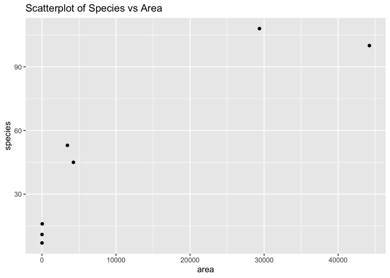
The relationship does not appear to be linear. We can check for the constant variance and normality of the data by plotting the distribution of residuals.
lm_island <- lm(species~area, data = islands)

head(lm_island$residuals)
## 1 2 3 4 5 6
## -17.403319 21.942004 11.990695 21.698674 -8.116835 -13.059832hist(lm_island$residuals)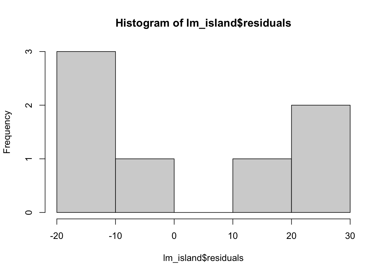
Or, alternatively with ggplot().
# create a data.frame which is required for ggplot
islands_res <- data.frame(residuals = lm_island$residuals)

ggplot(data = islands_res) +
  aes(x = residuals) +
  geom_histogram() +
  xlab("Residuals") +
  ggtitle("Histogram of Residuals")
## `stat_bin()` using `bins = 30`. Pick better value with `binwidth`.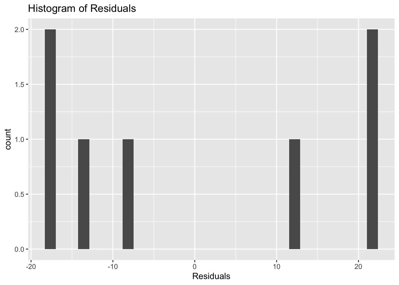
These residuals do not appear to be normally distributed.
We can also check the normality of the predictor variable, area, to see if transformation might be helpful. NOTE: Our predictor variables are often non-normal such as when we have a binary treatment vs control variable. Our concern is primarily with the assumptions of a linear relationship between \(Y\) and \(X\) and the assumption of normally distributed errors (residuals).
ggplot(data = islands) +
  aes(x = area) +
  geom_histogram()
## `stat_bin()` using `bins = 30`. Pick better value with `binwidth`.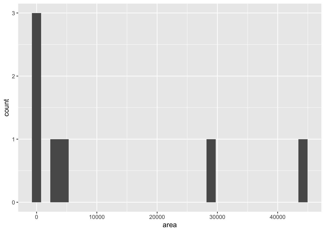
This plot shows that both outcome and predictor variables are non-normal, and so both might benefit from some kind of transformation. The researchers propose a log transformation of both variables.
# Carrying out log transformations
islands <- islands %>%
  dplyr::mutate(
    log_area = log(area),
    log_species = log(species)
  )

# Plotting transformed variables
ggplot(data = islands) +
  aes(x = log_area,
      y = log_species) +
  geom_point() +
  ggtitle("Scatterplot of log(Species) vs log(Area)") +
  geom_smooth(method = lm, se=FALSE)
## `geom_smooth()` using formula 'y ~ x'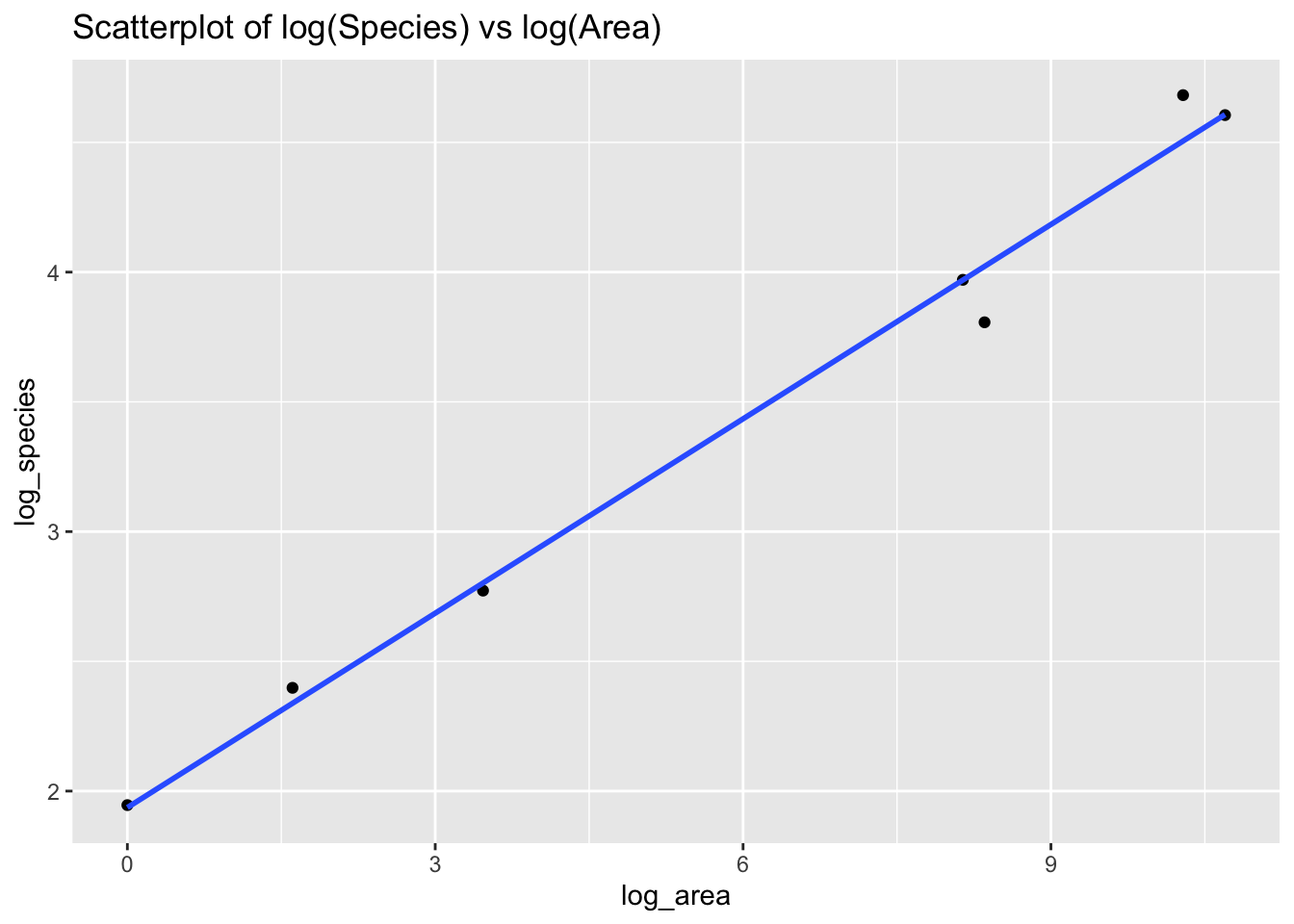
We fit a linear model on the logged variables.
10.4.1 Simple Linear Regression with Logged Variables
Here, the model is: \[ \hat{\mu}[log(Species) | log(Area)] = \beta_0 + \beta_1 * log(Area) \]
# Creating linear model
lm1 <- lm(log_species ~ log_area, data = islands)
summary(lm1)
##
## Call:
## lm(formula = log_species ~ log_area, data = islands)
##
## Residuals:
## 1 2 3 4 5 6 7
## -0.0021358 0.1769753 -0.2154872 0.0009468 -0.0292440 0.0595428 0.0094020
##
## Coefficients:
## Estimate Std. Error t value Pr(>|t|)
## (Intercept) 1.93651 0.08813 21.97 3.62e-06 ***
## log_area 0.24968 0.01211 20.62 4.96e-06 ***
## ---
## Signif. codes: 0 '***' 0.001 '**' 0.01 '*' 0.05 '.' 0.1 ' ' 1
##
## Residual standard error: 0.1283 on 5 degrees of freedom
## Multiple R-squared: 0.9884, Adjusted R-squared: 0.9861
## F-statistic: 425.3 on 1 and 5 DF, p-value: 4.962e-06Using stargazer():
# Remember to specify " results='asis' " when calling the chunk that includes stargazer()

# Creating table
stargazer(lm1,
          title = "log(Species) vs log(Area)",
          type = 'html',
header = FALSE)| Dependent variable: | |
| log_species | |
| log_area | 0.250*** |
| (0.012) | |
| Constant | 1.937*** |
| (0.088) | |
| Observations | 7 |
| R2 | 0.988 |
| Adjusted R2 | 0.986 |
| Residual Std. Error | 0.128 (df = 5) |
| F Statistic | 425.303*** (df = 1; 5) |
| Note: | p<0.1; p<0.05; p<0.01 |
And so, our estimated model is: \[ \hat \mu[log(Species) | log(Area)] = 1.937 + 0.250 * log(Area) \]
But because these are estimates, we have confidence intervals, which are:
# Calculating confidence interval on estimates
confint(lm1)
## 2.5 % 97.5 %
## (Intercept) 1.709959 2.1630569
## log_area 0.218558 0.280801810.4.2 Interpreting the Results
If \(\hat\mu[log(Y)|log(X)] = \beta_0 + \beta_1 log(X)\), then \(Median[Y|X] = e^{\beta_0} X^{\beta_1}\). So the doubling effect is (\(2^{\beta_1}\)).
And so, the 95% confidence interval of the multiplicative effect on the median of the number of species is:
# Calculating 95% confidence interval
2^confint(lm1)
## 2.5 % 97.5 %
## (Intercept) 3.271516 4.478628
## log_area 1.163570 1.214870Thus, our model estimates that doubling the area of the island is associated with 1.19 (\(2^{0.25}\); conf int: (1.16, 3.27)) times enlarging of the median of the number of species.
We can check some of the linear model assumptions now.
10.4.3 Assessment of Assumptions
R has four diagnostic plots that it can generate automatically with something like plot(lm_output):
1. Residuals vs Fitted: do residuals exhibit non-linear patterns?
2. Normal Q-Q: are residuals are normally distributed?
3. Scale-Location: are residuals are spread equally?
4. Cook’s distance: are some observations especially influential?
For more detail, see: https://data.library.virginia.edu/diagnostic-plots/
After we log-transformed the data, the distribution of observations become more normal.
# Plotting residual vs. fitted plot
plot(lm1, which = 1)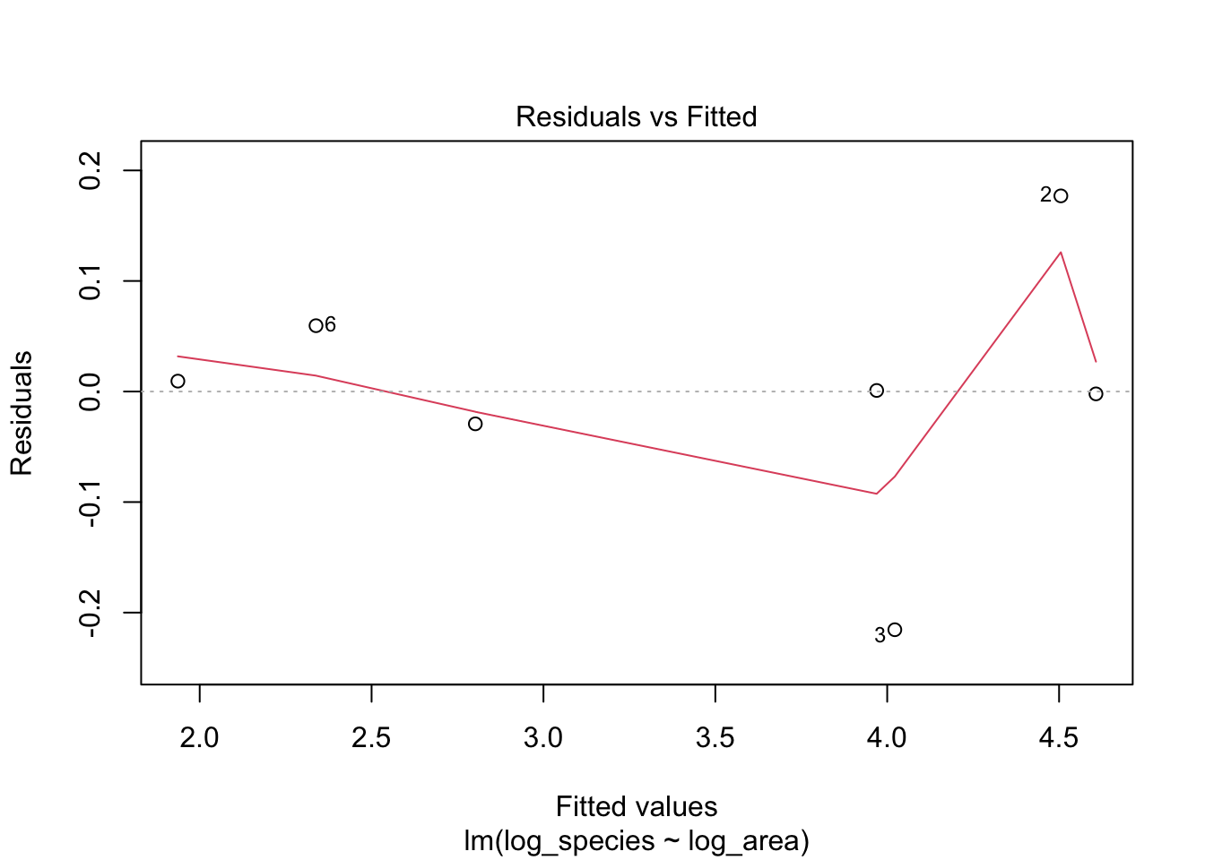
# Plotting normal Q-Q plot
plot(lm1, which = 2)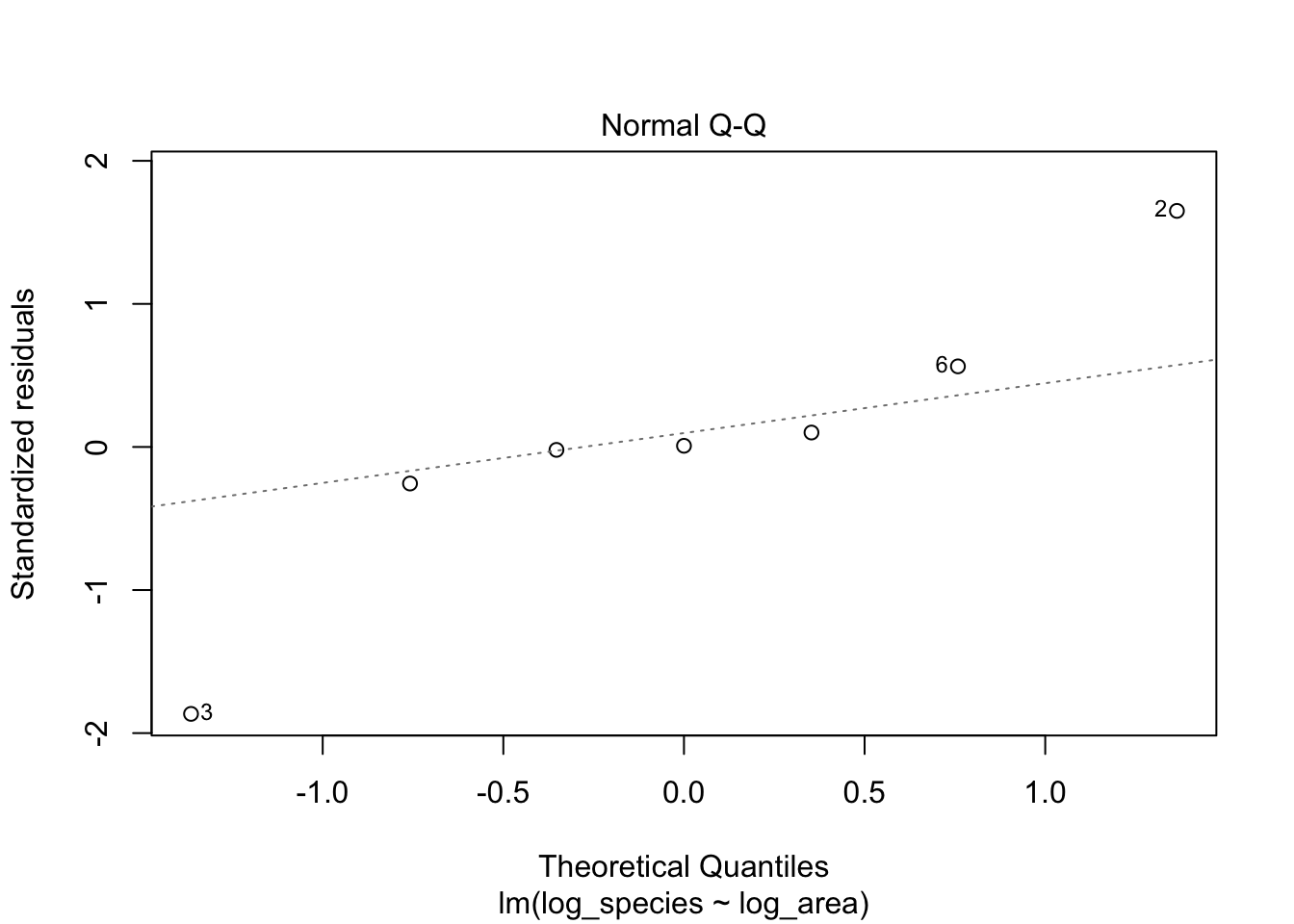
# Plotting
plot(lm1, which = 3)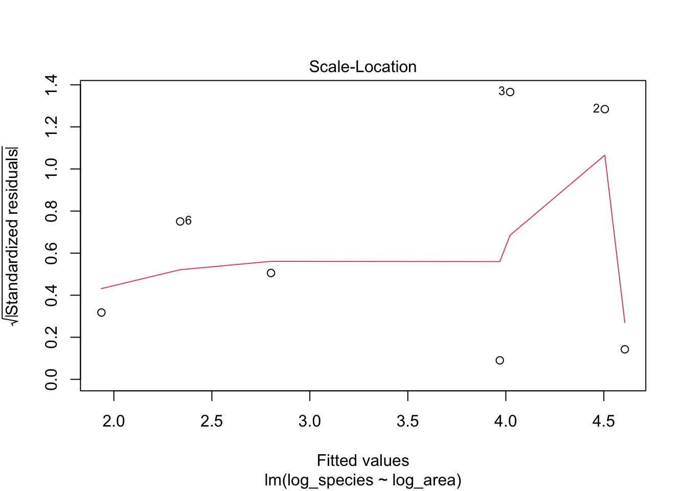
# Plotting
plot(lm1, which = 4)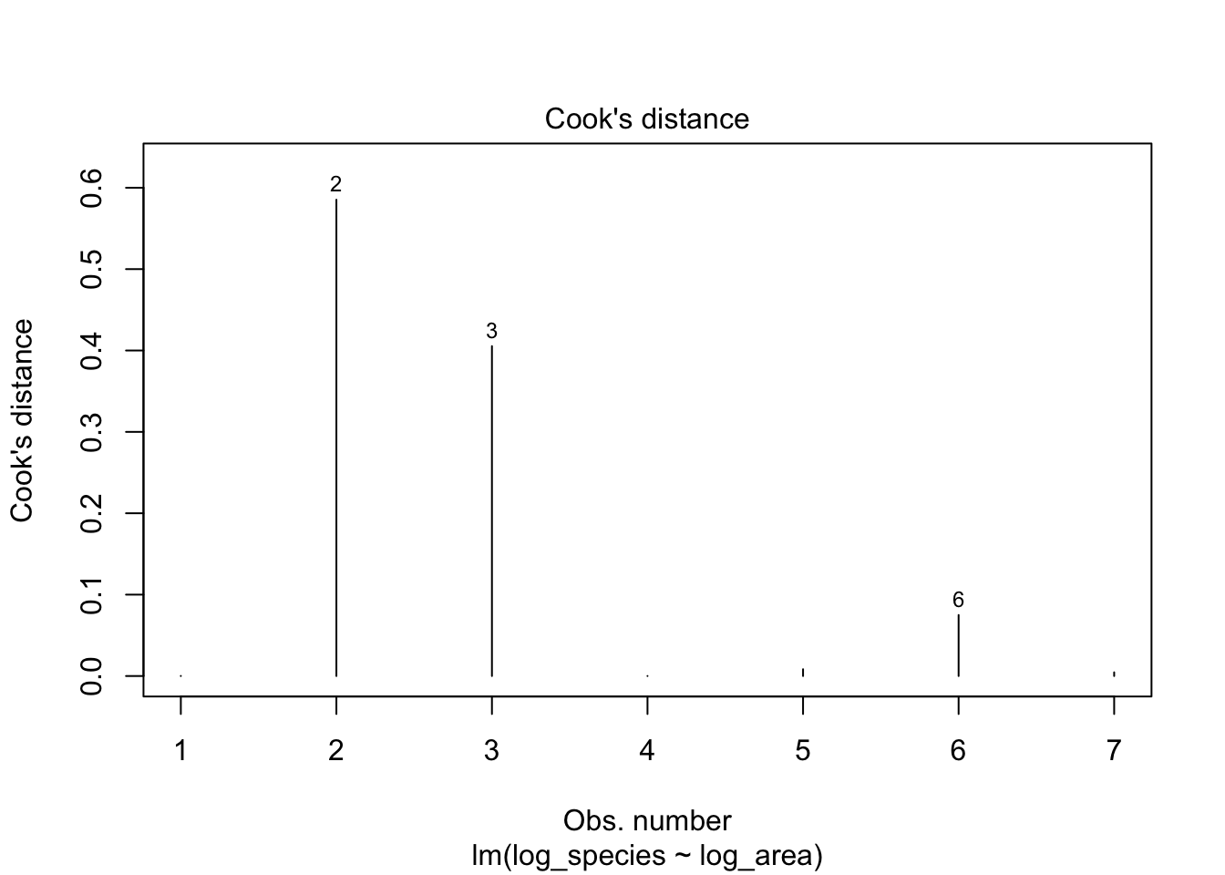
This supplement was put together by Omar Wasow, Sukrit S. Puri, and Blaykyi Kenyah. It builds on prior work by Project Mosaic, an “NSF-funded initiative to improve the teaching of statistics, calculus, science and computing in the undergraduate curriculum.” We are grateful to Nicholas Horton, Linda Loi, Kate Aloisio, and Ruobing Zhang for their effort developing The Statistical Sleuth in R.(horton2013statistical?)