Chapter 11 Multiple Regression
Supplement to chapter 9 of Ramsey and Schafer’s Statistical Sleuth 3ED for POL90: Statistics.
11.1 Effects of light on meadowfoam flowering
Do different amounts of light affect the growth of meadowfoam (a small plant used to create seed oil)? This is the question addressed in Case Study 9.1 in Statistical Sleuth 3e, Chapter 9, p 238.
Meadowfoam (Limnanthes alba) is a small plant found growing in moist meadows of the U.S. Pacific Northwest. It has been domesticated at Oregon State University for its seed oil, which is unique among vegetable oils for its long carbon strings. Like the oil from sperm whales, it is nongreasy and highly stable.
Researchers reported the results from one study in a series designed to find out how to elevate meadowfoam production to a profitable crop. In a controlled growth chamber, they focused on the effects of two light-related factors: light intensity, at the six levels of 150, 300, 450, 600, 750, and 900\(\mu\)mol/m2/sec; and the timing of the onset of the light treatment, either at photoperiodic floral induction (PFI)- the time at which the photo period was increased from 8 to 16 hours per day to induce flowering-or 24 days before PFI. The experimental design is depicted in Display 9.1. (Data from M. Seddigh and G. D. Jolliff, “Light Intensity Effects on Meadowfoam Growth and Flowering,” Crop Science 34 (1994): 497-503.)
11.1.1 Data coding, summary statistics and graphical display
We begin by loading packages, setting some display preferences, reading in the data, transforming some variables, and glancing at the data.
library(Sleuth3)
library(ggplot2)
library(dplyr)
library(stargazer)
library(xtable)
library(kableExtra)
library(janitor)

# Configure ggplot to theme_bw & larger type
theme_set(theme_bw(base_size = 18))

options(digits=3)
meadow <- Sleuth3::case0901 %>% clean_names()
meadow <- meadow %>%
mutate(time = ifelse(time > 1, "Early", "Late") %>% factor())
head(meadow)## flowers time intensity
## 1 62.3 Late 150
## 2 77.4 Late 150
## 3 55.3 Late 300
## 4 54.2 Late 300
## 5 49.6 Late 450
## 6 61.9 Late 450A total of 24 meadowfoam plants were included in this data. There were 12 treatment groups - 6 light intensities at each of the 2 timing levels (Display 9.2, page 239 of the Sleuth).
ggplot(data = meadow) +
  aes(x = intensity,
      y = flowers) +
  geom_point() +
  geom_smooth(method = "lm", se = FALSE) +
  labs(x = "light intensity (mu mol/m^2/sec)",
       y = "average number of flowers")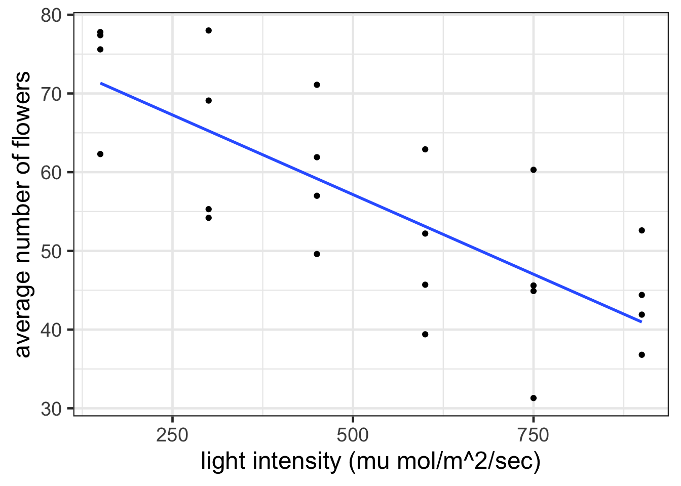
The following code generates the scatterplot of the average number of flowers per plant versus the applied light intensity for each of the 12 experimental units akin to Display 9.3 on page 240.
ggplot(data = meadow) +
  aes(x = intensity,
      y = flowers,
      color = time) +
  geom_point() +
  geom_smooth(method = "lm", se = FALSE) +
  labs(x = "light intensity (mu mol/m^2/sec)",
       y = "average number of flowers")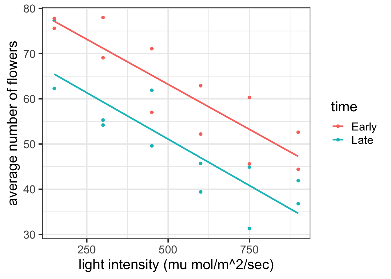
11.1.2 Multiple linear regression model
We next fit a multiple linear regression model that specifies parallel regression lines for the mean number of flowers as a function of light intensity as interpreted on page 239.
lm1 <- lm(flowers ~ intensity + time, data = meadow)

confint(lm1, level=.95) %>% # 95% confidence intervals
kable() | 2.5 % | 97.5 % | |
|---|---|---|
| (Intercept) | 76.656 | 90.27 |
| intensity | -0.051 | -0.03 |
| timeLate | -17.627 | -6.69 |
stargazer(lm1,
          header = FALSE,
type = 'html')| Dependent variable: | |
| flowers | |
| intensity | -0.040*** |
| (0.005) | |
| timeLate | -12.200*** |
| (2.630) | |
| Constant | 83.500*** |
| (3.270) | |
| Observations | 24 |
| R2 | 0.799 |
| Adjusted R2 | 0.780 |
| Residual Std. Error | 6.440 (df = 21) |
| F Statistic | 41.800*** (df = 2; 21) |
| Note: | p<0.1; p<0.05; p<0.01 |
We can also fit a multiple linear regression with an interaction between light intensity and timing of its initiation as shown in Display 9.14 (page 260) and interpreted on page 239.
lm2 <- lm(flowers ~ intensity * time, data = meadow)

stargazer(lm1, lm2,
          header = FALSE,
type = 'html')| Dependent variable: | ||
| flowers | ||
| (1) | (2) | |
| intensity | -0.040*** | -0.040*** |
| (0.005) | (0.007) | |
| timeLate | -12.200*** | -11.500* |
| (2.630) | (6.140) | |
| intensity:timeLate | -0.001 | |
| (0.011) | ||
| Constant | 83.500*** | 83.100*** |
| (3.270) | (4.340) | |
| Observations | 24 | 24 |
| R2 | 0.799 | 0.799 |
| Adjusted R2 | 0.780 | 0.769 |
| Residual Std. Error | 6.440 (df = 21) | 6.600 (df = 20) |
| F Statistic | 41.800*** (df = 2; 21) | 26.500*** (df = 3; 20) |
| Note: | p<0.1; p<0.05; p<0.01 | |
The model with the interaction term does not appear to have substantively different coefficients than the model without the interaction term. We can confirm that the addition of an additional term (the interaction term) does not add much explanatory power by running an ANOVA test.
anova(lm1, lm2) %>%
kable()| Res.Df | RSS | Df | Sum of Sq | F | Pr(>F) |
|---|---|---|---|---|---|
| 21 | 871 | NA | NA | NA | NA |
| 20 | 871 | 1 | 0.576 | 0.013 | 0.91 |
The small \(F\)-statistic and large \(p\)-value confirm that the reduced model (no interaction term) is preferable to the full model (with interaction term).
11.1.3 Statistical Conclusion
Display 9.3 shows the fit of a multiple linear regression model that specifies paral- lel regression lines for the mean number of flowers as functions of light intensity. Increasing light intensity decreased the mean number of flowers per plant by an estimated 4.0 flowers per plant per 100 \(\mu\)mol/m2 /sec (953 confidence interval from 3.0 to 5.1). Beginning the light treatments 24 days prior to PFI increased the mean numbers of flowers by an estimated 12.2 flowers per plant (953 confidence interval from 6.7 to 17.6). The data provide no evidence that the effect of light intensity depends on the timing of its initiation (two-sided p-value = 0.91, from at-test for interaction, 20 degrees of freedom).
11.2 Why do some mammals have large brains?
What characteristics predict large brains in mammals? This is the question addressed in Case Study 9.2 in Statistical Sleuth 3e, Chapter 9, p 239.
Evolutionary biologists are keenly interested in the characteristics that enable a species to withstand the selective mechanisms of evolution. An interesting variable in this respect is brain size. One might expect that bigger brains are better, but certain penalties seem to be associated with large brains, such as the need for longer pregnancies and fewer offspring. Although the individual members of the large- brained species may have more chance of surviving, the benefits for the species must be good enough to compensate for these penalties. To shed some light on this issue, it is helpful to determine exactly which characteristics are associated with large brains, after getting the effect of body size out of the way.
The data in Display 9.4 are the average values of brain weight, body weight, gestation lengths (length of pregnancy), and litter size for 96 species of mammals. (Data from G. A. Sacher and E. F. Staffeldt, “Relation of Gestation Time to Brain Weight for Placental Mammals; Implications for the Theory of Vertebrate Growth,’’ American Naturalist, 108 (1974): 593-613. The common names for the species cor- respond to the Latin names given in the original paper, and those followed by a Roman numeral indicate subspecies.) Since brain size is obviously related to body size, the question of interest is this: Which, if any, variables are·associated with brain size, after accounting for body size?
11.2.1 Data coding and summary statistics
mammals <- Sleuth3::case0902 %>% clean_names()

mammals <- mammals %>%
  mutate(log_brain  = log(brain),
         log_body   = log(body),
         log_gest   = log(gestation),
         log_litter = log(litter))

head(mammals)
## species brain body gestation litter log_brain log_body log_gest
## 1 Aardvark 9.6 2.20 31 5.0 2.26 0.788 3.43
## 2 Acouchis 9.9 0.78 98 1.2 2.29 -0.248 4.58
## 3 African elephant 4480.0 2800.00 655 1.0 8.41 7.937 6.48
## 4 Agoutis 20.3 2.80 104 1.3 3.01 1.030 4.64
## 5 Axis deer 219.0 89.00 218 1.0 5.39 4.489 5.38
## 6 Badger 53.0 6.00 60 2.2 3.97 1.792 4.09
## log_litter
## 1 1.609
## 2 0.182
## 3 0.000
## 4 0.262
## 5 0.000
## 6 0.788A total of 96 mammals were included in this data. The average values of brain weight, body weight, gestation length, and litter size for each of the species were calculated and presented in Display 9.4 (page 241 of the Sleuth).
11.2.2 Graphical presentation
The following displays a simple (unadorned) pairs plot, akin to Display 9.10 on page 255.
mammals_small <- mammals %>%
  dplyr::select(brain, body, gestation, litter)

pairs(mammals_small)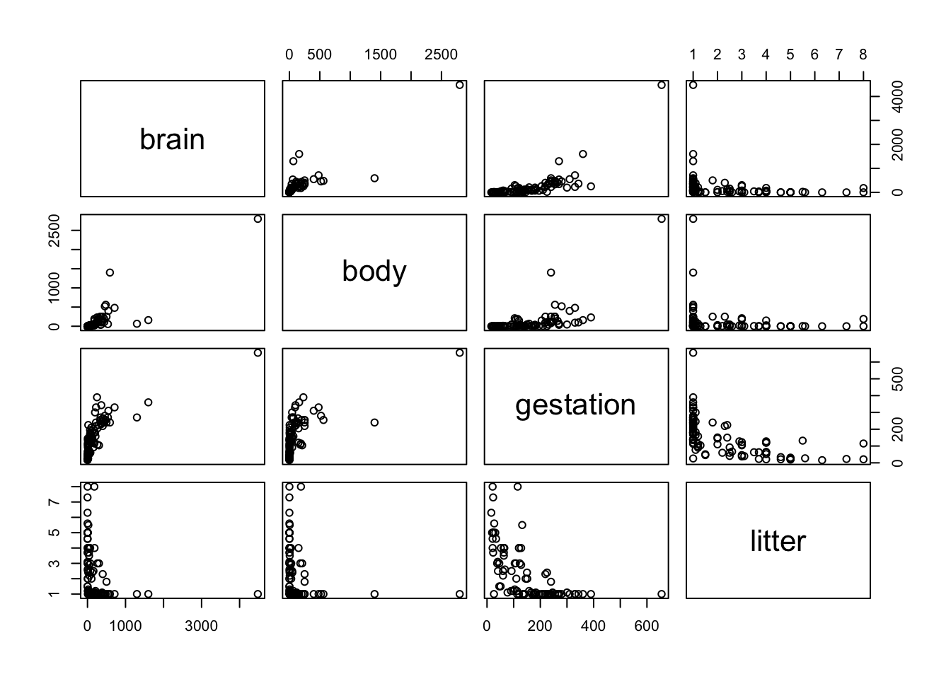
The following displays a jittered scatterplot of log brain weight as a function of log litter size, akin to Display 9.12 on page 258.
ggplot(data = mammals) +
  aes(x = log_litter,
      y = log_brain) +
  geom_point(alpha = 0.5) + # alpha makes points somewhat transparent
  geom_smooth(method = "lm", se = FALSE)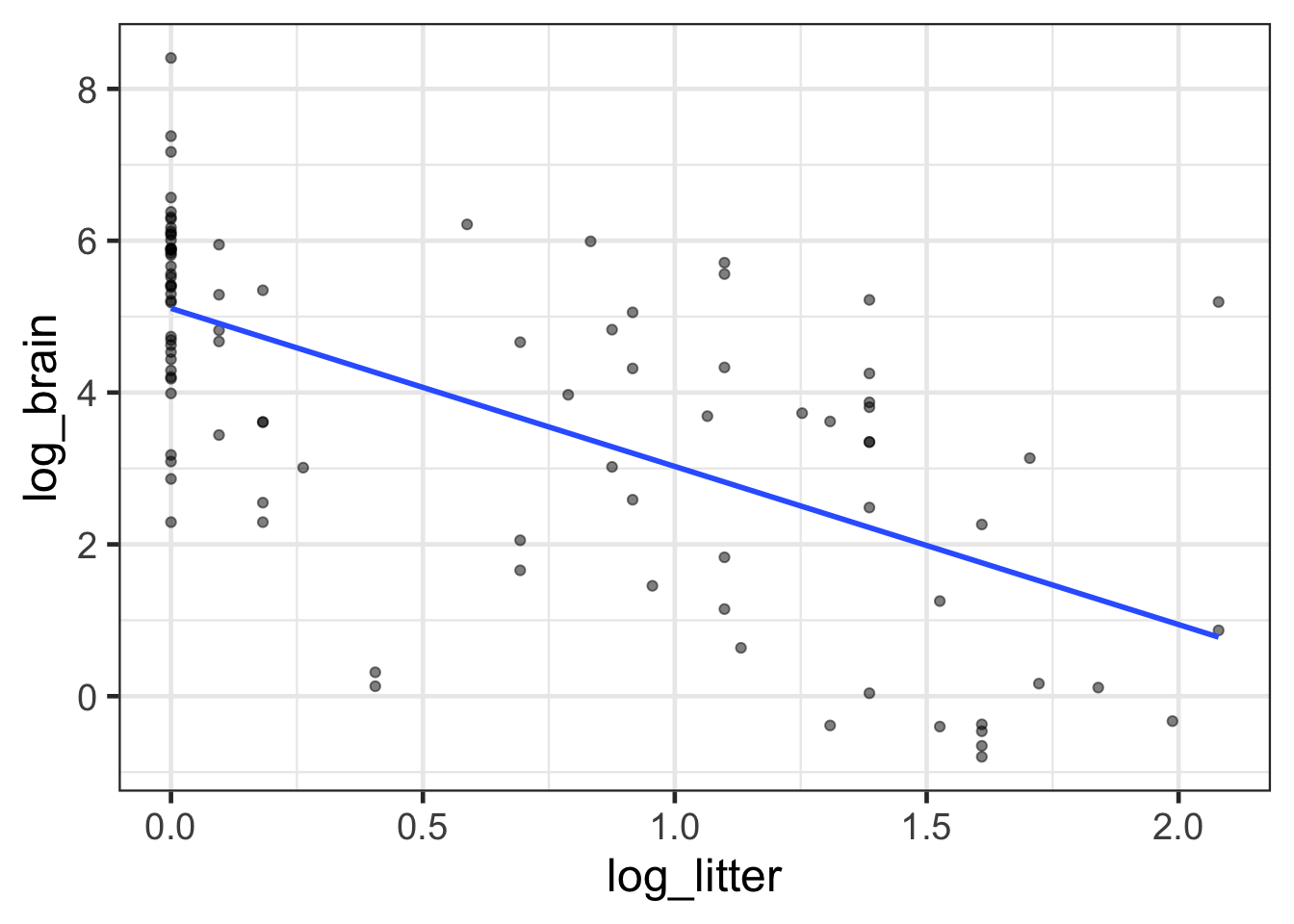
Below displays a jittered scatterplot using the original data on a log-transformed axis, akin to Display 9.12 on page 258.
ggplot(data = mammals) +
  aes(x = litter,
      y = brain) +
    geom_point(alpha = 0.5) +
    geom_smooth(method = "lm", se = FALSE) +
    scale_x_log10() +
    scale_y_log10()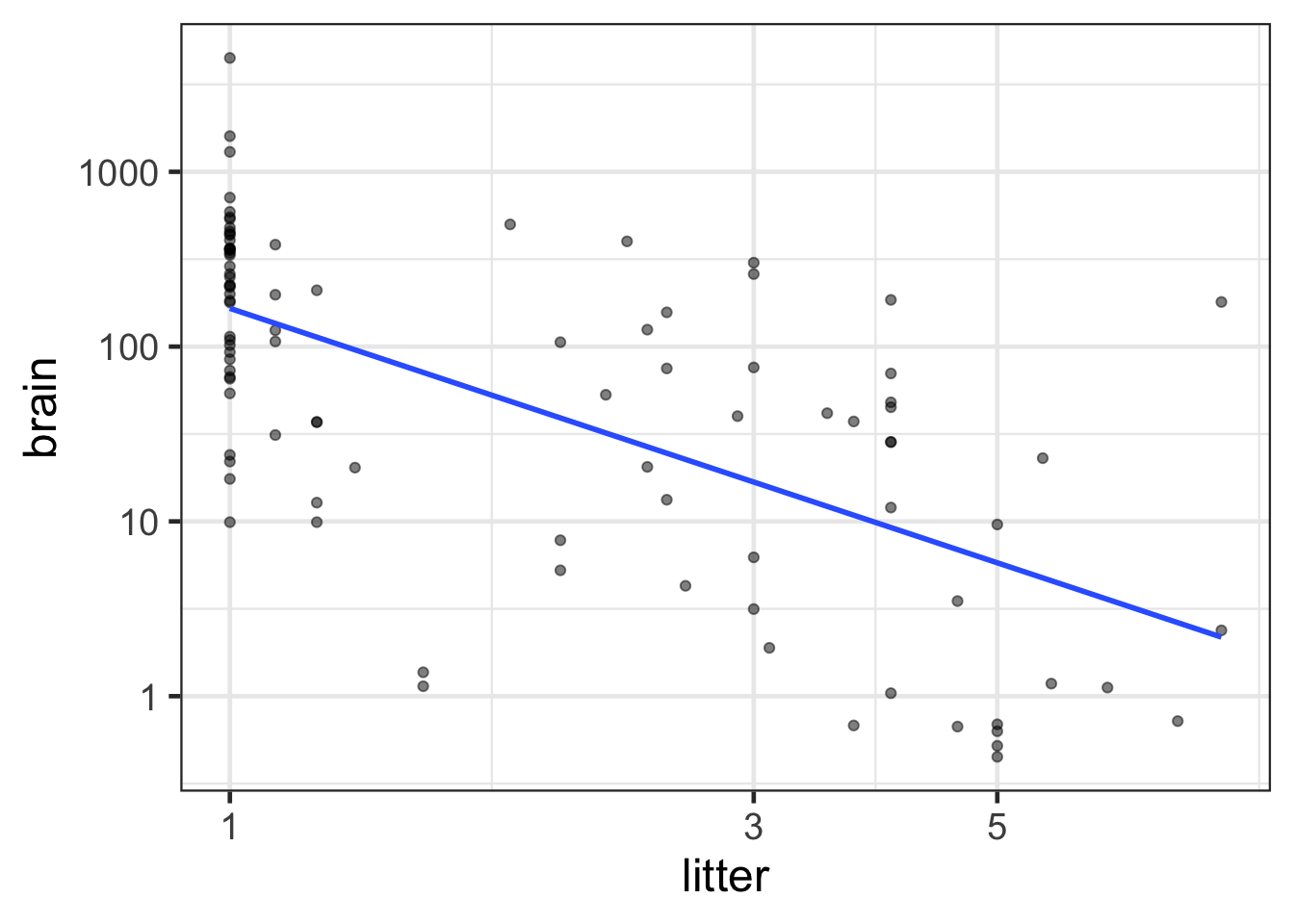
The following displays a jittered scatterplot using the original data stratified by body weight on a log-transformed axis, akin to Display 9.13 on page 259.
mammals$weightcut <- cut(mammals$body, breaks=c(0, 2.1, 9.1, 100, 4200),
                         labels=c("Body Weight: 0kg to 2.1kg",
                                  "Body Weight: 2.1kg to 9.1kg",
                                  "Body Weight: 9.1kg to 100kg",
                                  "Body Weight: 100 to 4,200"))

ggplot(data = mammals) +
  aes(x = litter,
      y = brain) +
    aes(x = litter,
      y = brain) +
    geom_point(alpha = 0.5) +
    geom_smooth(method = "lm", se = FALSE) +
    scale_x_log10() +
    scale_y_log10() +
  facet_wrap(~ weightcut)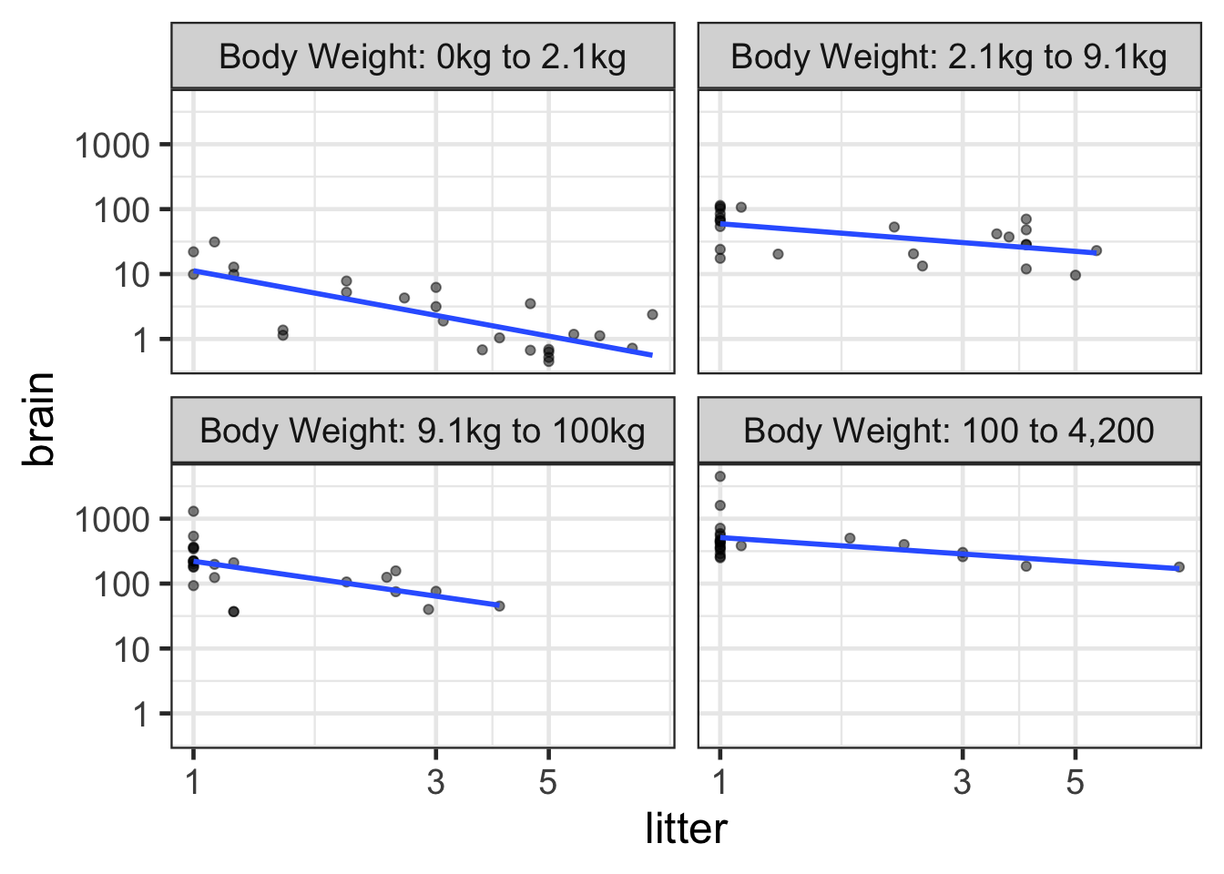
11.2.3 Multiple linear regression model
The following model is interpreted on page 240 and shown in Display 9.15 (page 260).
lm1 <- lm(log_brain ~ log_body + log_gest + log_litter, data = mammals)

stargazer(lm1,
          header = FALSE,
type = 'html')| Dependent variable: | |
| log_brain | |
| log_body | 0.575*** |
| (0.033) | |
| log_gest | 0.418*** |
| (0.141) | |
| log_litter | -0.310*** |
| (0.116) | |
| Constant | 0.855 |
| (0.662) | |
| Observations | 96 |
| R2 | 0.954 |
| Adjusted R2 | 0.952 |
| Residual Std. Error | 0.475 (df = 92) |
| F Statistic | 632.000*** (df = 3; 92) |
| Note: | p<0.1; p<0.05; p<0.01 |
11.2.4 Statistical Conclusion
The data provide convincing evidence that brain weight was associated with either gestation length or litter size, even after accounting for the effect of body weight (\(p\)-value < 0.0001; extra sum of squares \(F\)-test). There was strong evidence that litter size was associated with brain weight after accounting for body weight and gestation (two-sided \(p\)-value = 0.0089) and that gestation period was associated with brain weight after accounting for body weight and litter size (two-sided \(p\)-value = 0.0038).
11.2.5 Scope ofInference
As suggestive as the findings may be, inferences that go beyond these data are unwise. The data were summarized from available studies and cannot be represen- tative of any wider population. As usual, no causal interpretation can be made from these observational data.
This supplement was put together by Omar Wasow. It builds on prior work by Project Mosaic, an “NSF-funded initiative to improve the teaching of statistics, calculus, science and computing in the undergraduate curriculum.” We are grateful to Nicholas Horton, Linda Loi, Kate Aloisio, and Ruobing Zhang for their effort developing The Statistical Sleuth in R.(horton2013statistical?)