Chapter 12 OLS with Polynomials and Interactions
Sample R code for Ramsey and Schafer’s Statistical Sleuth 3ed for POL90: Statistics.
12.1 Introduction
This document is intended to help describe how to undertake analyses introduced as examples in the Second Edition of the Statistical Sleuth (2002) by Fred Ramsey and Dan Schafer. More information about the book can be found at. This file as well as the associated reproducible analysis source file can be found at .
We also set some options to improve legibility of graphs and output.
trellis.par.set(theme=col.mosaic())  # get a better color scheme for lattice
options(digits=3)
The specific goal of this document is to demonstrate how to calculate the quantities described in Chapter 10: Inferential Tools for Multiple Regression using R.
12.2 Galileo’s data on the motion of falling bodies
Galileo investigated the relationship between height and horizontal distance. This is the question addressed in case study 10.1 in the Sleuth.
12.2.1 Data coding, summary statistics and graphical display
We begin by reading the data and summarizing the variables.
galileo <- Sleuth3::case1001
summary(galileo)
## Distance Height
## Min. :253 Min. : 100
## 1st Qu.:366 1st Qu.: 250
## Median :451 Median : 450
## Mean :434 Mean : 493
## 3rd Qu.:514 3rd Qu.: 700
## Max. :573 Max. :1000head(galileo, 2)## Distance Height
## 1 253 100
## 2 337 200There we a total of 7 trials of Galileo’s experiment. For each trial, he recorded the initial height and then measured the horizontal distance as shown in Display 10.1 (page 268).
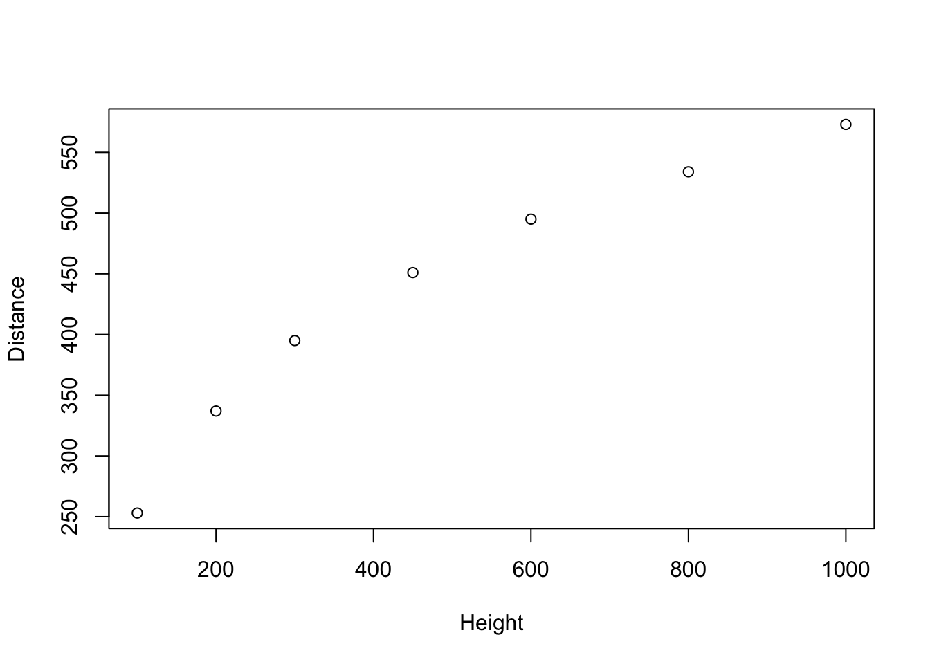
We can start to explore this relationship by creating a scatterplot of Galileo’s horizontal distances versus initial heights. The following graph is akin to Display 10.2 (page 269).
plot(Distance ~ Height, data=galileo)
12.2.2 2.2 Models
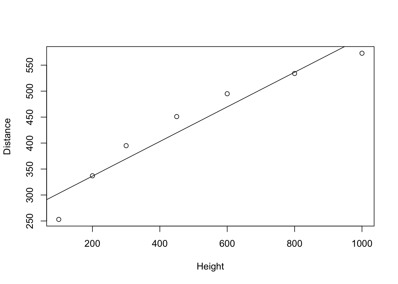
The first model that we created is a cubic model as interpreted on page 269 and summarized in Display 10.13 (page 286).
lm0 <- lm(Distance ~ Height, data=galileo)
summary(lm0)
##
## Call:
## lm(formula = Distance ~ Height, data = galileo)
##
## Residuals:
## 1 2 3 4 5 6 7
## -50.05 0.62 25.29 31.29 25.29 -2.38 -30.05
##
## Coefficients:
## Estimate Std. Error t value Pr(>|t|)
## (Intercept) 269.712 24.312 11.09 0.00010 ***
## Height 0.333 0.042 7.93 0.00051 ***
## ---
## Signif. codes: 0 '***' 0.001 '**' 0.01 '*' 0.05 '.' 0.1 ' ' 1
##
## Residual standard error: 33.7 on 5 degrees of freedom
## Multiple R-squared: 0.926, Adjusted R-squared: 0.912
## F-statistic: 62.9 on 1 and 5 DF, p-value: 0.000513plot(Distance ~ Height, data=galileo)
abline(lm0)
lm1 <- lm(Distance ~ Height+I(Height^2) + I(Height^3),
          data=galileo)
summary(lm1)
##
## Call:
## lm(formula = Distance ~ Height + I(Height^2) + I(Height^3), data = galileo)
##
## Residuals:
## 1 2 3 4 5 6 7
## -2.4036 3.5809 1.8917 -4.4688 -0.0804 2.3216 -0.8414
##
## Coefficients:
## Estimate Std. Error t value Pr(>|t|)
## (Intercept) 1.56e+02 8.33e+00 18.71 0.00033 ***
## Height 1.12e+00 6.57e-02 16.98 0.00044 ***
## I(Height^2) -1.24e-03 1.38e-04 -8.99 0.00290 **
## I(Height^3) 5.48e-07 8.33e-08 6.58 0.00715 **
## ---
## Signif. codes: 0 '***' 0.001 '**' 0.01 '*' 0.05 '.' 0.1 ' ' 1
##
## Residual standard error: 4.01 on 3 degrees of freedom
## Multiple R-squared: 0.999, Adjusted R-squared: 0.999
## F-statistic: 1.6e+03 on 3 and 3 DF, p-value: 2.66e-05We next decrease the polynomial for Height by one degree to obtain a quadratic model as interpreted on page 269 and summarized in Display 10.7 (page 277). This model is used for most of the following results.
lm2 <- lm(Distance ~ Height+I(Height^2), data=galileo)
summary(lm2)
##
## Call:
## lm(formula = Distance ~ Height + I(Height^2), data = galileo)
##
## Residuals:
## 1 2 3 4 5 6 7
## -14.31 9.17 13.52 1.94 -6.18 -12.61 8.46
##
## Coefficients:
## Estimate Std. Error t value Pr(>|t|)
## (Intercept) 2.00e+02 1.68e+01 11.93 0.00028 ***
## Height 7.08e-01 7.48e-02 9.47 0.00069 ***
## I(Height^2) -3.44e-04 6.68e-05 -5.15 0.00676 **
## ---
## Signif. codes: 0 '***' 0.001 '**' 0.01 '*' 0.05 '.' 0.1 ' ' 1
##
## Residual standard error: 13.6 on 4 degrees of freedom
## Multiple R-squared: 0.99, Adjusted R-squared: 0.986
## F-statistic: 205 on 2 and 4 DF, p-value: 9.33e-05We can fit an equivalent model (with different parametrization) using the function:
lmpoly <- lm(Distance ~ poly(Height, 5), data=galileo)
summary(lmpoly)
##
## Call:
## lm(formula = Distance ~ poly(Height, 5), data = galileo)
##
## Residuals:
## 1 2 3 4 5 6 7
## 0.1594 -0.7323 1.1159 -0.9275 0.4882 -0.1196 0.0159
##
## Coefficients:
## Estimate Std. Error t value Pr(>|t|)
## (Intercept) 434.000 0.646 671.93 0.00095 ***
## poly(Height, 5)1 267.116 1.709 156.31 0.00407 **
## poly(Height, 5)2 -70.194 1.709 -41.08 0.01550 *
## poly(Height, 5)3 26.378 1.709 15.44 0.04118 *
## poly(Height, 5)4 -5.960 1.709 -3.49 0.17777
## poly(Height, 5)5 3.132 1.709 1.83 0.31794
## ---
## Signif. codes: 0 '***' 0.001 '**' 0.01 '*' 0.05 '.' 0.1 ' ' 1
##
## Residual standard error: 1.71 on 1 degrees of freedom
## Multiple R-squared: 1, Adjusted R-squared: 1
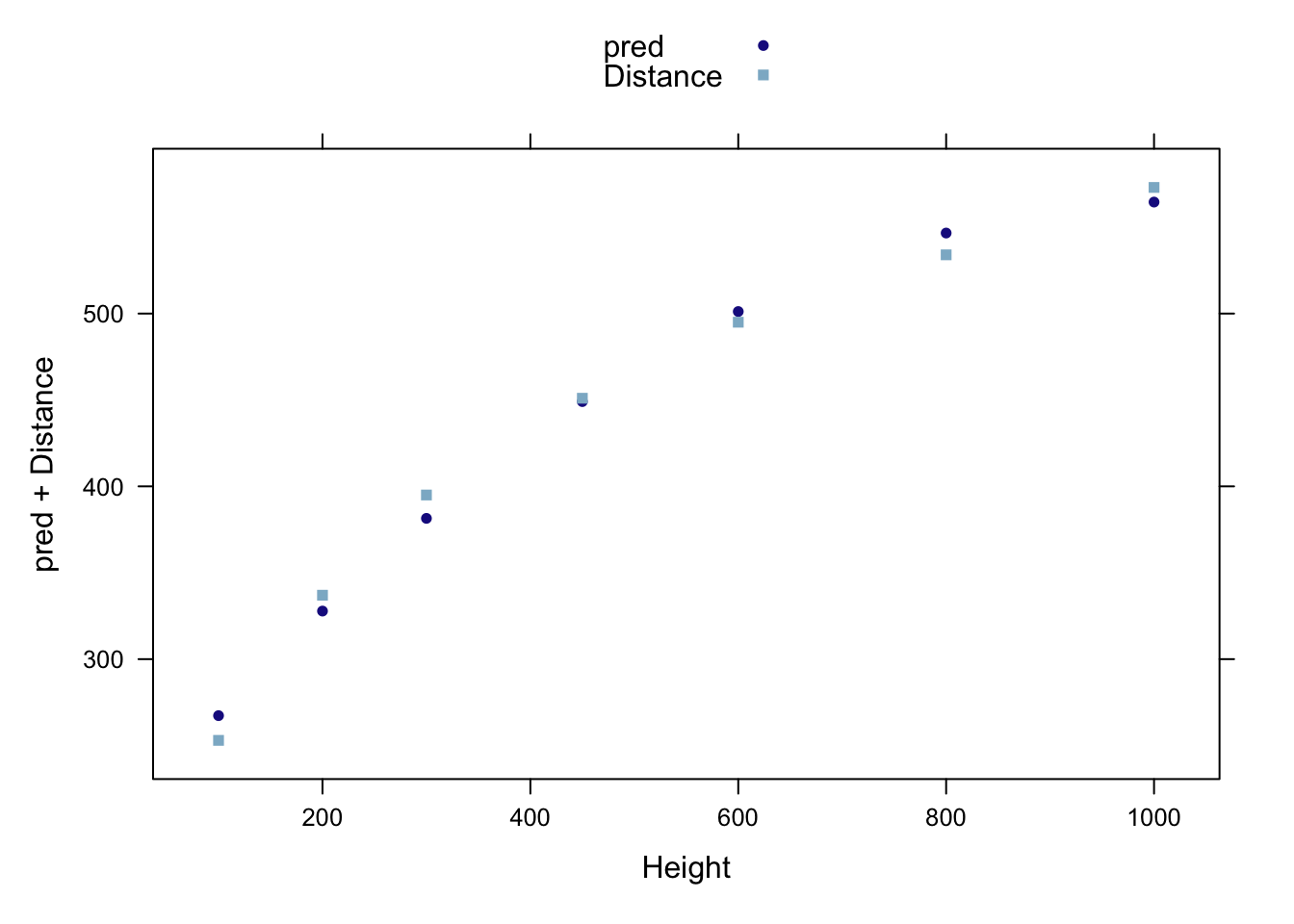
## F-statistic: 5.27e+03 on 5 and 1 DF, p-value: 0.0105The following figure presents the predicted values from the quadratic model and the original data points akin to Display 10.2 (page 269).
galileo <- transform(galileo, pred = predict(lm2))
xyplot(pred+Distance ~ Height, auto.key=TRUE, data=galileo)
To obtain the expected values of \(\hat{\mu}\left(\mathrm{Distance}|\mathrm{Height} = 0 \right)\) and \(\hat{\mu}\left(\mathrm{Distance}|\mathrm{Height} = 250\right)\), we used the command with the quadratic model as shown in Display 10.7 (page 277).
predict(lm2, interval="confidence", data.frame(Height=c(0, 250)))## fit lwr upr
## 1 200 153 246
## 2 356 337 374We can also verify the above confidence interval calculations with the following code:
355.1+c(-1, 1)*6.62*qt(.975, 4)## [1] 337 373To verify numbers on page 279, an interval for the predicted values , we used the following code:
predict(
    lm2,
    interval="predict",
    data.frame(Height=c(0, 250))
    )
## fit lwr upr
## 1 200 140 260
## 2 356 313 398Lastly, we display the ANOVA table for the quadratic model that is interpreted on page 283 (Display 10.11).
anova(lm2) %>%
    xtable() %>%
        print(type = "html",
comment = FALSE) # turn off message about package| Df | Sum Sq | Mean Sq | F value | Pr(>F) | |
|---|---|---|---|---|---|
| Height | 1 | 71350.79 | 71350.79 | 383.57 | 0.0000 |
| I(Height^2) | 1 | 4927.13 | 4927.13 | 26.49 | 0.0068 |
| Residuals | 4 | 744.08 | 186.02 |
12.3 3 Echolocation in bats
How do bats make their way about in the dark? Echolocation requires a lot of energy. Does it depend on mass and species? This is the question addressed in case study 10.2 in the Sleuth.
12.3.1 Data coding, summary statistics and graphical display
We begin by reading the data, performing transformations where necessary and summarizing the variables.
bats <- Sleuth3::case1002
bats <- transform(bats, logmass = log(Mass))
bats <- transform(bats, logenergy = log(Energy))
head(bats,2)
## Mass Type Energy logmass logenergy
## 1 779 non-echolocating bats 43.7 6.66 3.78
## 2 628 non-echolocating bats 34.8 6.44 3.55A total of nrow(bats) flying vertebrates were included in this study. There were nrow(subset(bats, Type=="echolocating bats")) echolocating bats, nrow(subset(bats, Type=="non-echolocating bats")) non-echolocating bats, and nrow(subset(bats, Type=="non-echolocating birds")) non-echolocating birds. For each subject their mass and flight energy expenditure were recorded as shown in Display 10.3
(page 270).
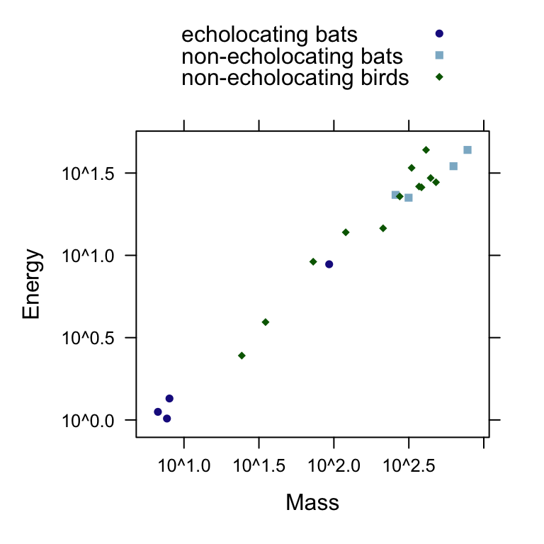
We can next observe the pattern between log(energy expenditure) as a function of log(body mass) for each group with a scatterplot. The following figure is akin to Display 10.4 (page 271).
xyplot(
    Energy ~ Mass,
    group=Type,
    scales=list(y=list(log=TRUE),
    x=list(log=TRUE)),
    auto.key=TRUE,
    data=bats
    )
12.3.2 2.1 Multiple regression
We first evaluate a multiple regression model for log(energy expenditure) given type of species and log(body mass) as defined on page 272 and shown in Display 10.6 (page 273).
lm1 <- lm(logenergy ~ logmass, data=bats)
#stargazer(lm0, type='html')
stargazer(lm1, type = 'html')| Dependent variable: | |
| logenergy | |
| logmass | 0.809*** |
| (0.027) | |
| Constant | -1.470*** |
| (0.137) | |
| Observations | 20 |
| R2 | 0.981 |
| Adjusted R2 | 0.979 |
| Residual Std. Error | 0.180 (df = 18) |
| F Statistic | 908.000*** (df = 1; 18) |
| Note: | p<0.1; p<0.05; p<0.01 |
lm2 <- lm(logenergy ~ logmass + Type, data=bats)
#summary(lm1)
stargazer(lm1, lm2, type='html')| Dependent variable: | ||
| logenergy | ||
| (1) | (2) | |
| logmass | 0.809*** | 0.815*** |
| (0.027) | (0.045) | |
| Typenon-echolocating bats | -0.079 | |
| (0.203) | ||
| Typenon-echolocating birds | 0.024 | |
| (0.158) | ||
| Constant | -1.470*** | -1.500*** |
| (0.137) | (0.150) | |
| Observations | 20 | 20 |
| R2 | 0.981 | 0.982 |
| Adjusted R2 | 0.979 | 0.978 |
| Residual Std. Error | 0.180 (df = 18) | 0.186 (df = 16) |
| F Statistic | 908.000*** (df = 1; 18) | 284.000*** (df = 3; 16) |
| Note: | p<0.1; p<0.05; p<0.01 | |
Next, we calculated confidence intervals for the coefficients which are interpreted on page 274.
confint(lm1)## 2.5 % 97.5 %
## (Intercept) -1.756 -1.180
## logmass 0.752 0.865exp(confint(lm1))## 2.5 % 97.5 %
## (Intercept) 0.173 0.307
## logmass 2.122 2.375Since the significance of a model depends on which variables are included, the Sleuth proposes two other models, one only looking at the type of flying animal and the other allows the three groups to have different straight-line regressions with mass. These two models are displayed below and discussed on pages 274–275.
summary(lm(logenergy ~ Type, data=bats))##
## Call:
## lm(formula = logenergy ~ Type, data = bats)
##
## Residuals:
## Min 1Q Median 3Q Max
## -1.8872 -0.3994 0.0236 0.4932 1.5253
##
## Coefficients:
## Estimate Std. Error t value Pr(>|t|)
## (Intercept) 0.653 0.422 1.55 0.14058
## Typenon-echolocating bats 2.743 0.597 4.59 0.00026 ***
## Typenon-echolocating birds 2.134 0.488 4.38 0.00041 ***
## ---
## Signif. codes: 0 '***' 0.001 '**' 0.01 '*' 0.05 '.' 0.1 ' ' 1
##
## Residual standard error: 0.845 on 17 degrees of freedom
## Multiple R-squared: 0.595, Adjusted R-squared: 0.548
## F-statistic: 12.5 on 2 and 17 DF, p-value: 0.000458summary(lm(logenergy ~ Type * logmass, data=bats))##
## Call:
## lm(formula = logenergy ~ Type * logmass, data = bats)
##
## Residuals:
## Min 1Q Median 3Q Max
## -0.2515 -0.1264 -0.0095 0.0812 0.3284
##
## Coefficients:
## Estimate Std. Error t value Pr(>|t|)
## (Intercept) -1.4705 0.2477 -5.94 3.6e-05 ***
## Typenon-echolocating bats 1.2681 1.2854 0.99 0.34
## Typenon-echolocating birds -0.1103 0.3847 -0.29 0.78
## logmass 0.8047 0.0867 9.28 2.3e-07 ***
## Typenon-echolocating bats:logmass -0.2149 0.2236 -0.96 0.35
## Typenon-echolocating birds:logmass 0.0307 0.1028 0.30 0.77
## ---
## Signif. codes: 0 '***' 0.001 '**' 0.01 '*' 0.05 '.' 0.1 ' ' 1
##
## Residual standard error: 0.19 on 14 degrees of freedom
## Multiple R-squared: 0.983, Adjusted R-squared: 0.977
## F-statistic: 163 on 5 and 14 DF, p-value: 6.7e-12To construct the confidence bands discussed on page 277 and shown in Display 10.9 (page 279) we used the following code:
pred <- predict(
    lm1,
    se.fit=TRUE,
    newdata=data.frame(
        Type=c("non-echolocating birds", "non-echolocating birds"),
        logmass=c(log(100), log(400))
        )
    )
pred.fit <- pred$fit[1]
pred.fit
## 1
## 2.26pred.se <- pred$se.fit[1]
pred.se## 1
## 0.0409multiplier <- sqrt(4*qf(.95, 4, 16));
multiplier## [1] 3.47lower <- exp(pred.fit-pred.se*multiplier)
lower## 1
## 8.28upper <- exp(pred.fit+pred.se*multiplier)
upper ## 1
## 11# for the other reference points
pred2 <- predict(
lm1,
se.fit=TRUE,
newdata=data.frame(
Type=c("non-echolocating bats", "non-echolocating bats"),
logmass=c(log(100), log(400))
)
)
pred3 <- predict(
lm1,
se.fit=TRUE,
newdata=data.frame(
Type=c("echolocating bats", "echolocating bats"),
logmass=c(log(100), log(400))
)
)
table10.9 <- rbind(
c("Intercept estimate", "Standard error"),
round(cbind(pred2$fit, pred2$se.fit), 4),
round(cbind(pred3$fit, pred3$se.fit), 4)
)
table10.9## [,1] [,2]
## "Intercept estimate" "Standard error"
## 1 "2.2555" "0.0409"
## 2 "3.3765" "0.05"
## 1 "2.2555" "0.0409"
## 2 "3.3765" "0.05"Next we can assess the model by evaluating the extra sums of squares \(F\)-test for testing the equality of intercepts in the parallel regression lines model as shown in Display 10.10 (page 282).
lm1 <- lm(logenergy ~ logmass, data=bats)
lm2 <- lm(logenergy ~ logmass + Type, data=bats)

anova(lm1, lm2) %>%
    xtable() %>%
    print(type = "html",
comment = FALSE) # turn off message about package| Res.Df | RSS | Df | Sum of Sq | F | Pr(>F) | |
|---|---|---|---|---|---|---|
| 1 | 18 | 0.58 | ||||
| 2 | 16 | 0.55 | 2 | 0.03 | 0.43 | 0.6593 |
We can also compare the full model with interaction terms and the reduced model (without interaction terms) with the extra sum of squares \(F\)-test as described in Display 10.12 (page 284).
lm3 <- lm(logenergy ~ logmass * Type, data=bats)
stargazer(lm1, lm2, lm3, type = 'html',
omit.stat = c("f", "ser"))| Dependent variable: | |||
| logenergy | |||
| (1) | (2) | (3) | |
| logmass | 0.809*** | 0.815*** | 0.805*** |
| (0.027) | (0.045) | (0.087) | |
| Typenon-echolocating bats | -0.079 | 1.270 | |
| (0.203) | (1.280) | ||
| Typenon-echolocating birds | 0.024 | -0.110 | |
| (0.158) | (0.385) | ||
| logmass:Typenon-echolocating bats | -0.215 | ||
| (0.224) | |||
| logmass:Typenon-echolocating birds | 0.031 | ||
| (0.103) | |||
| Constant | -1.470*** | -1.500*** | -1.470*** |
| (0.137) | (0.150) | (0.248) | |
| Observations | 20 | 20 | 20 |
| R2 | 0.981 | 0.982 | 0.983 |
| Adjusted R2 | 0.979 | 0.978 | 0.977 |
| Note: | p<0.1; p<0.05; p<0.01 | ||
anova(lm2, lm3) %>%
    xtable() %>%
    print(type = "html",
comment = FALSE) # turn off message about package| Res.Df | RSS | Df | Sum of Sq | F | Pr(>F) | |
|---|---|---|---|---|---|---|
| 1 | 16 | 0.55 | ||||
| 2 | 14 | 0.50 | 2 | 0.05 | 0.67 | 0.5265 |
anova(lm1, lm2, lm3) %>%
    xtable() %>%
    print(type = "html",
comment = FALSE) # turn off message about package| Res.Df | RSS | Df | Sum of Sq | F | Pr(>F) | |
|---|---|---|---|---|---|---|
| 1 | 18 | 0.58 | ||||
| 2 | 16 | 0.55 | 2 | 0.03 | 0.41 | 0.6713 |
| 3 | 14 | 0.50 | 2 | 0.05 | 0.67 | 0.5265 |
This supplement was put together by Omar Wasow. It builds on prior work by Project Mosaic, an “NSF-funded initiative to improve the teaching of statistics, calculus, science and computing in the undergraduate curriculum.” We are grateful to Nicholas Horton, Linda Loi, Kate Aloisio, and Ruobing Zhang for their effort developing The Statistical Sleuth in R.(horton2013statistical?)