Logistic Regression for Binary Response Variables
knitr::opts_chunk$set(echo = TRUE)
Survival in the Donner Party–An Observational Study
From Statistical Sleuth, Chapter 20 (p 602, 3e):
In 1846 the Donner and Reed families left Springfield, Illinois, for California by covered wagon. In July, the Donner Party, as it became known, reached Fort Bridger, Wyoming. There its leaders decided to attempt a new and untested route to the Sacramento Valley. Having reached its full size of 87 people and 20 wagons, the party was delayed by a difficult crossing of the Wasatch Range and again in the crossing of the desert west of the Great Salt Lake. The group became stranded in the eastern Sierra Nevada mountains when the region was hit by heavy snows in late October. By the time the last survivor was rescued on April 21, 1847, 40 of the 87 members had died from famine and exposure to extreme cold.
These data were used by an anthropologist to study the theory that females are better able to withstand harsh conditions than are males. (Data from D. K. Grayson, “Donner Party Deaths: A Demographic Assessment,” Journal of Anthropological Research 46 (1990): 223-42.) For any given age, were the odds of survival greater for women than for men?
Statistical Conclusion
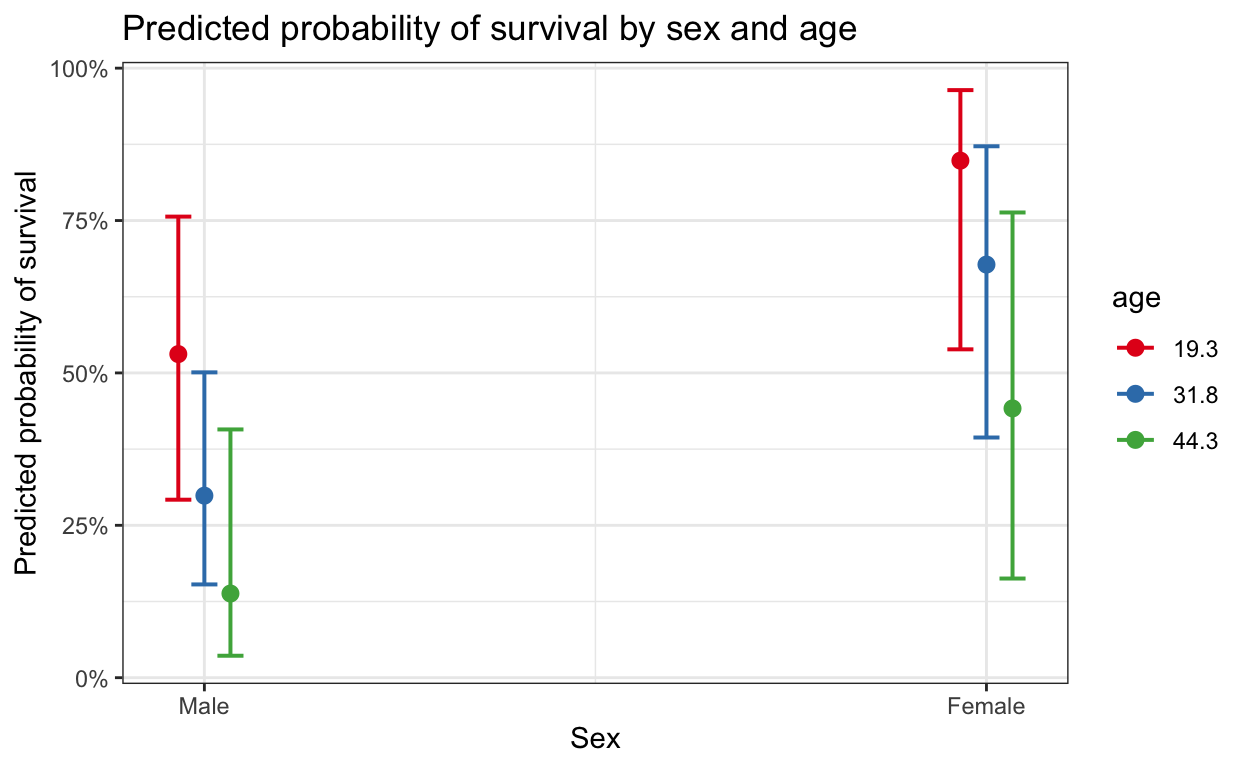
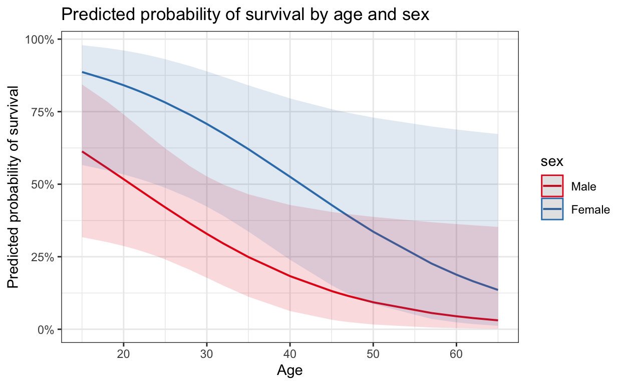
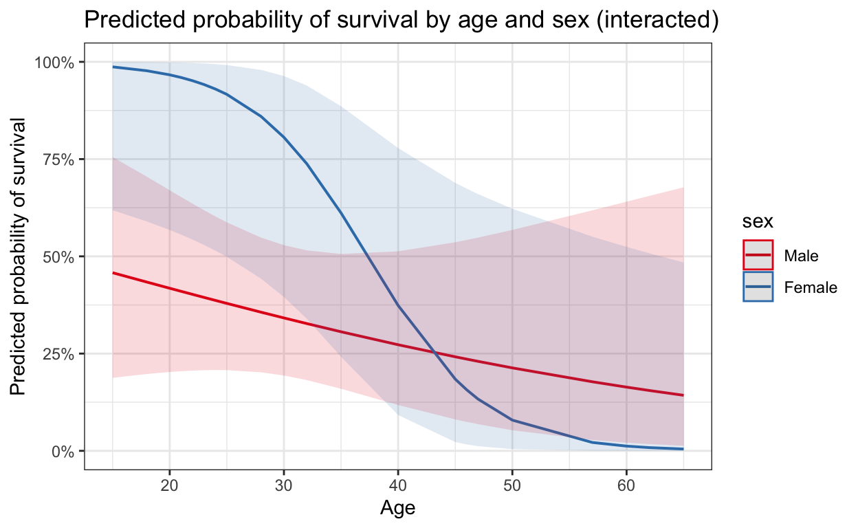
While it generally appears that older adults were less likely than younger adults to survive, the data provide highly suggestive evidence that the age effect is more pronounced for females than for males (the two-sided p-value for interaction of gender and age is 0.05). Ignoring the interaction leads to an informal conclusion about the overall difference between men and women: The data provide highly suggestive evidence that the survival probability was higher for women (in the Donner Party) than for the men (two-sided p-value = 0.02 from a drop-in-deviance test). The odds of survival for women are estimated to be 5 times the odds of survival for similarly aged men (95% confidence interval: 1.2 times to 25.2 times, from a drop-in-deviance-based confidence interval).
Scope of Inference
Since the data are observational, the result cannot be used as proof that women were more apt to survive than men; the possibility of confounding variables cannot be excluded. Furthermore, since the 45 individuals were not drawn at random from any population, inference to a broader population is not justified.
Load packages and data
# load data
donner <- Sleuth3::case2001 %>%
  clean_names()

# convert Survived/Died to ones/zeros
donner <- donner %>%
  mutate(survived = as.numeric(status == "Survived"),
         sex = fct_relevel(sex, c("Male", "Female"))) # male = reference category

# view data
head(donner)
  age    sex   status survived
1  23   Male     Died        0
2  40 Female Survived        1
3  40   Male Survived        1
4  30   Male     Died        0
5  28   Male     Died        0
6  40   Male     Died        0
# create regression table
stargazer(glm_sex, glm_age, glm_sa, glm_int,
type = 'html',
header = FALSE)
| Dependent variable: | ||||
| survived | ||||
| (1) | (2) | (3) | (4) | |
| sexFemale | 1.390** | 1.600** | 6.930** | |
| (0.671) | (0.755) | (3.400) | ||
| age | -0.066** | -0.078** | -0.032 | |
| (0.032) | (0.037) | (0.035) | ||
| sexFemale:age | -0.162* | |||
| (0.094) | ||||
| Constant | -0.693* | 1.820* | 1.630 | 0.318 |
| (0.387) | (0.999) | (1.110) | (1.130) | |
| Observations | 45 | 45 | 45 | 45 |
| Log Likelihood | -28.600 | -28.100 | -25.600 | -23.700 |
| Akaike Inf. Crit. | 61.300 | 60.300 | 57.300 | 55.300 |
| Note: | p<0.1; p<0.05; p<0.01 | |||
Explaining results
From Statistical Sleuth, (p 608, 3e)
The fit of a logistic regression model to the Donner Party data, where \(\pi\) represents survival probability, gives \[ logit(\hat{\pi}) = 1.63 - 0.078 \times age + 1.60 \times female \] For comparing women 50 years old (A) with women 20 years old (B), the odds ratio is estimated to be exp[-0.078(50 - 20)] = 0.096, or about 1/10. So the odds of a 20-year-old woman surviving were about 10 times the odds of a 50-year-old woman surviving. Comparing a woman (\(female\) = 1 = A) with a man (\(female\) = 0 = B) of the same age, the estimated odds ratio is exp(1.60[1 - 0) = 4.95—a woman’s odds were about 5 times the odds of survival of a man of the same age.
Comparing models
# for ANOVA with logistic regression, need to specify test = "Chisq"
anova(glm_sex, glm_sa, test = "Chisq") %>%
  xtable() %>%
    print(type = "html",
        comment = FALSE) # turn off message about package
| Resid. Df | Resid. Dev | Df | Deviance | Pr(>Chi) | |
|---|---|---|---|---|---|
| 1 | 43 | 57.29 | |||
| 2 | 42 | 51.26 | 1 | 6.03 | 0.0141 |
# for ANOVA with logistic regression, need to specify test = "Chisq"
anova(glm_sa, glm_int, test = "Chisq") %>%
  xtable() %>%
    print(type = "html",
        comment = FALSE) # turn off message about package
| Resid. Df | Resid. Dev | Df | Deviance | Pr(>Chi) | |
|---|---|---|---|---|---|
| 1 | 42 | 51.26 | |||
| 2 | 41 | 47.35 | 1 | 3.91 | 0.0480 |
Visualizing models
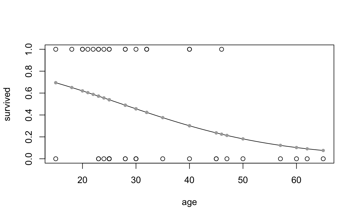
Look at survival vs age with base R.
# plot with base R
x_age <- seq(15, 65, by = 1)
y_status <- predict(glm_age, list(age = x_age), type="response")

plot(data = donner,
     survived ~ age)
lines(x_age, y_status)
points(donner$age, fitted(glm_age), pch=20, col = "darkgrey")
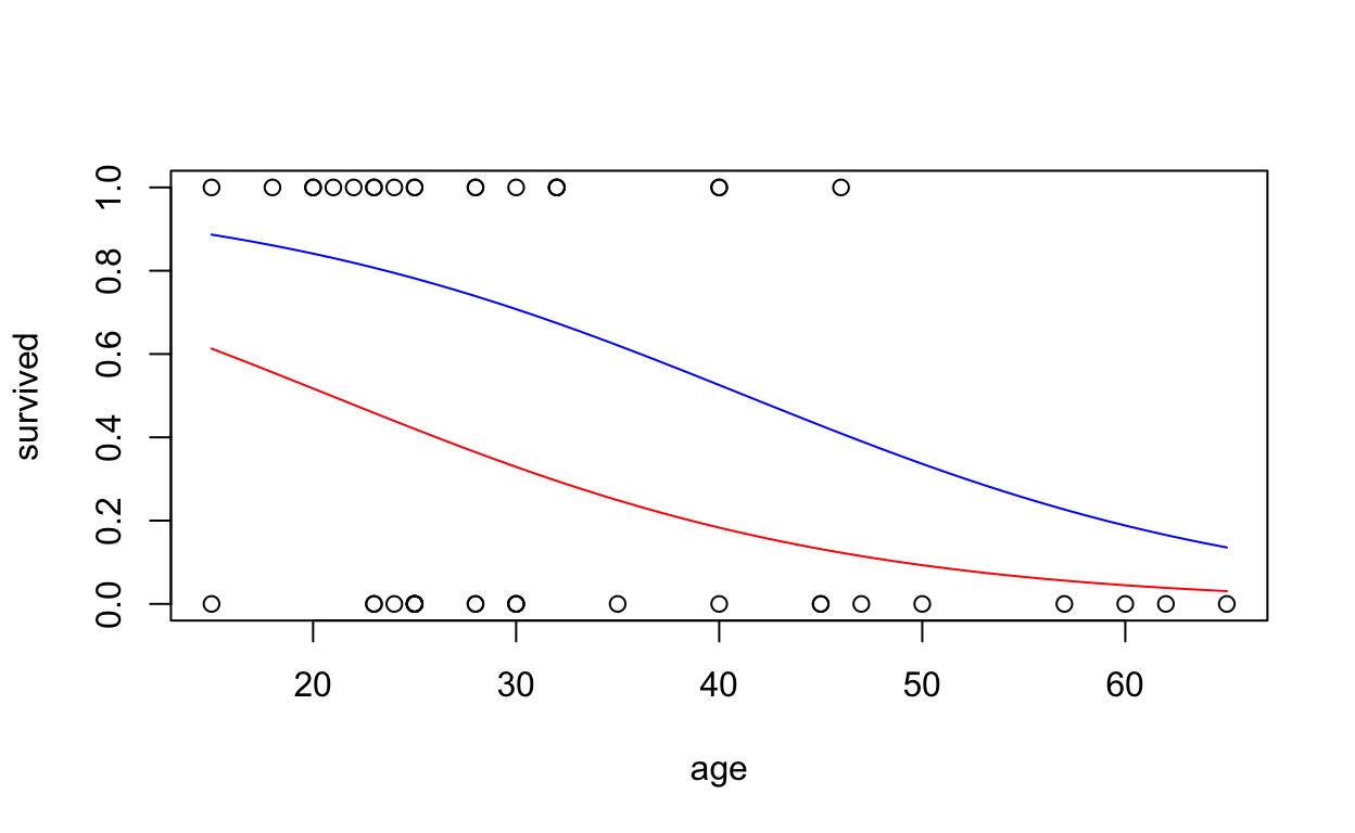
# plot with base R, by sex
x_age <- seq(15, 65, by = 1)
x_male <- rep("Male", length(x_age))
x_female <- rep("Female", length(x_age))

y_pred_male   <- predict(glm_sa, list(age = x_age, sex = x_male), type="response")
y_pred_female <- predict(glm_sa, list(age = x_age, sex = x_female), type="response")

plot(survived ~ age, data = donner)

lines(x_age, y_pred_male, col = "red")
lines(x_age, y_pred_female, col = "blue")
Marginal effects
With simple linear regression using two variables, plotting the relationship between some \(Y\) against some \(X\) is trivial. With multiple regression, however, it is typically difficult to plot multiple dimensions in 2D. Similarly, more complicated models, such as those with interaction terms or non-linear relationships as in logistic regression can be harder to interpret and plot.
One solution is to estimate marginal or partial effects that tell us how an outcome variable changes when an explanatory variable changes while other explanatory variables are held constant.
In R there are a growing number of ways to estimate and
plot marginal effects. To start, we’ll use the margins
package with the Donner data and a multivariable model.
    factor     AME     SE       z      p   lower   upper
       age -0.0153 0.0060 -2.5504 0.0108 -0.0270 -0.0035
 sexFemale  0.3258 0.1356  2.4028 0.0163  0.0601  0.5916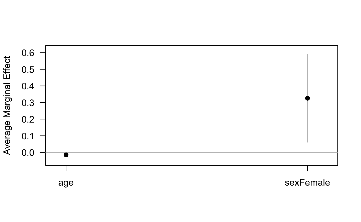
Marginal effects with
sjPlot
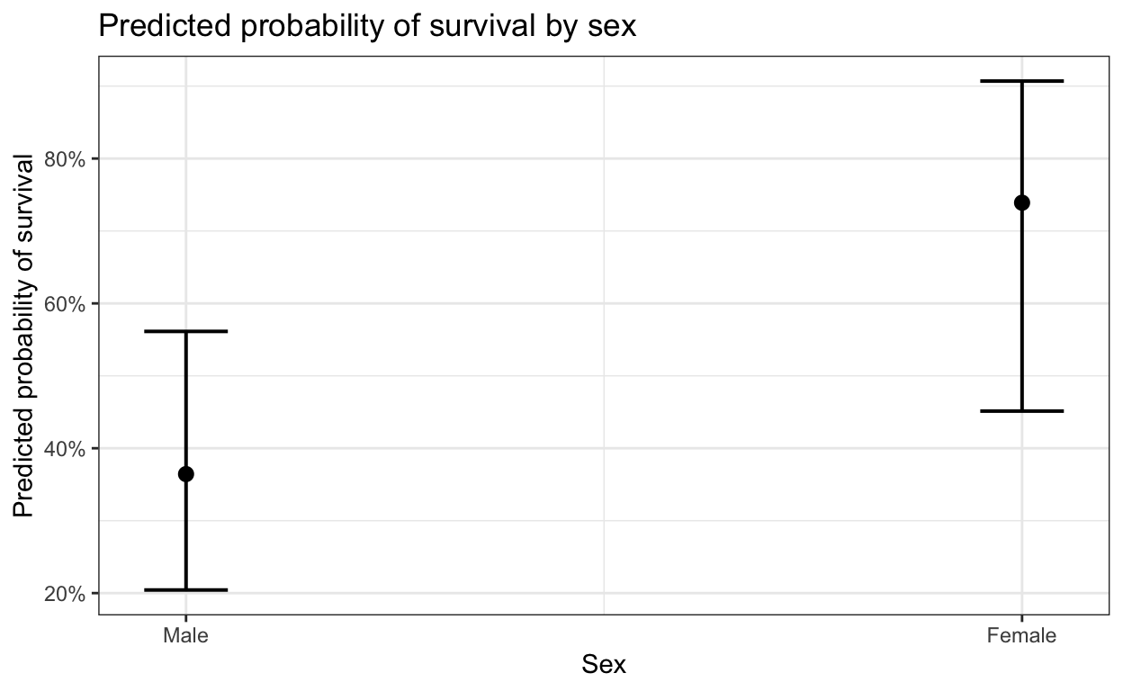
The sjPlot package offers a plot_model
command which offers a number of options to easily plot predicted
probabilities from logistic regression models.
# with sjPlot package
# https://cran.r-project.org/web/packages/sjPlot/vignettes/plot_marginal_effects.html

# with binary or discrete predictors, use type = "eff"
plot_model(glm_sa, type = "eff", terms = "sex") +
  ggtitle("Predicted probability of survival by sex") +
  ylab("Predicted probability of survival") +
  xlab("Sex")
# adding second variable
# with binary or discrete predictors, use type = "eff"
plot_model(glm_sa, type = "eff", terms = c("sex", "age")) +
  ggtitle("Predicted probability of survival by sex and age") +
  ylab("Predicted probability of survival") +
  xlab("Sex")
# change x-axis
# with continuous predictor on x-axis, use type = "pred"
plot_model(glm_sa, type = "pred",
           terms = c("age [15, 25, 35, 45, 55, 65]", "sex")) +
  ggtitle("Predicted probability of survival by age and sex") +
  ylab("Predicted probability of survival") +
  xlab("Age")

# change x-axis
# with continuous predictor on x-axis, use type = "pred"
plot_model(glm_sa, type = "pred",
           terms = c("age [all]", "sex")) +
  ggtitle("Predicted probability of survival by age and sex") +
  ylab("Predicted probability of survival") +
  xlab("Age")
# plot interaction model
# with continuous predictor on x-axis, use type = "pred"
plot_model(glm_int, type = "pred",
           terms = c("age [all]", "sex")) +
  ggtitle("Predicted probability of survival by age and sex (interacted)") +
  ylab("Predicted probability of survival") +
  xlab("Age")
Summary of findings
While it generally appears that older adults were less likely than younger adults to survive, the data provide highly suggestive evidence that the age effect is more pronounced for females than for males (the two-sided \(p\)-value for interaction of gender and age is 0.05). Ignoring the interaction leads to an informal conclusion about the overall difference between men and women: The data provide highly suggestive evidence that the survival probability was higher for women (in the Donner Party) than for the men (two-sided \(p\)-value = 0.02 from a drop-in-deviance test). The odds of survival for women are estimated to be 5 times the odds of survival for similarly aged men (95% confidence interval: 1.2 times to 25.2 times, from a drop-in-deviance-based confidence interval).
Since the data are observational, the result cannot be used as proof that women were more apt to survive than men; the possibility of confounding variables cannot be excluded. Furthermore, since the 45 individuals were not drawn at random from any population, inference to a broader population is not justified.
Birdkeeping and Lung Cancer–A Retrospective Observational Study
From Statistical Sleuth, Chapter 20, (p 602-3, 3e)
A 1972-1981 health survey in The Hague, Netherlands, discovered an association between keeping pet birds and increased risk of lung cancer. To investigate bird- keeping as a risk factor, researchers conducted a case-control study of patients in 1985 at four hospitals in The Hague (population 450,000). They identified 49 cases of lung cancer among patients who were registered with a general practice, who were age 65 or younger, and who had resided in the city since 1965. They also selected 98 controls from a population of residents having the same general age structure. (Data based on P.A. Holst, D. Kromhout, and R. Brand, “For Debate: Pet Birds as an Independent Risk Factor for Lung Cancer,’’ British Medical Journal 297 (1988): 13-21.)
Age and smoking history are both known to be associated with lung cancer incidence. After age, socioeconomic status, and smoking have been controlled for, is an additional risk associated with birdkeeping?
Statistical Conclusion
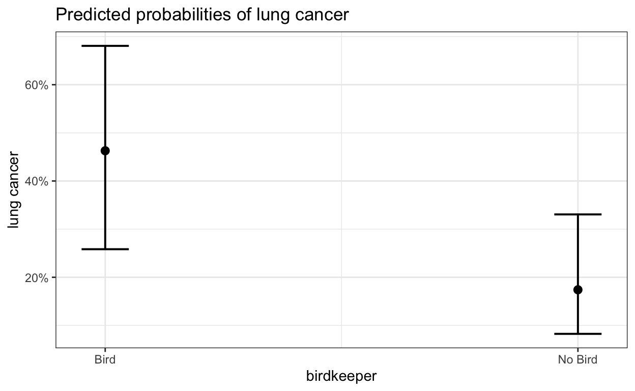
The odds of lung cancer among birdkeepers are estimated to be 3.8 times as large as the odds of lung cancer among nonbirdkeepers, after accounting for the effects of smoking, sex, age, and socioeconomic status. An approximate 95% confidence interval for this odds ratio is 1.7 to 8.5. The data provide convincing evidence that increased odds of lung cancer were associated with keeping pet birds, even after accounting for the effect of smoking (one-sided \(p\)-value = 0.0008).
Scope of Inference
Inference extends to the population of lung cancer patients and unaffected individu- als in The Hague in 1985. Statistical analysis of these observational data cannot be used as evidence that birdkeeping causes the excess cancer incidence among bird- keepers, although the data are consistent with that theory. (As further evidence in support of the causal theory, the researchers investigated other potential confound- ing variables [beta-carotene intake, vitamin C intake, and alcohol consumption]. They also cited medical rationale supporting the statistical associations: People who keep birds inhale and expectorate excess allergens and dust particles, increasing the likelihood of dysfunction of lung macrophages, which in turn can lead to diminished immune system response.)
Code book
- FM = Sex(1 = F, 0 = M)
- AG = Age, in years
- SS = Socioeconomic status (1 = High, 0 = Low), determined by occupation of the household’s principal wage earner
- YR = Years of smoking prior to diagnosis or examination
- CD = Average rate of smoking, in cigarettes per day
- BK = Indicator of birdkeeping (caged birds in the home for more than 6 consecutive months from 5 to 14 years before diagnosis (cases) or examination (controls)
# load data
birds <- Sleuth3::case2002 %>%
  clean_names()

birds <- birds %>%
  mutate(lung_cancer = as.numeric(lc == "LungCancer")) %>%
  rename(birdkeeper = bk,
    years_smoking = yr)


head(birds)
          lc   fm   ss birdkeeper ag years_smoking cd lung_cancer
1 LungCancer Male  Low       Bird 37            19 12           1
2 LungCancer Male  Low       Bird 41            22 15           1
3 LungCancer Male High     NoBird 43            19 15           1
4 LungCancer Male  Low       Bird 46            24 15           1
5 LungCancer Male  Low       Bird 49            31 20           1
6 LungCancer Male High NoBird 51 24 15 1stargazer(glm_bk, glm_bk2,
type = 'html',
header = FALSE)
| Dependent variable: | ||
| lung_cancer | ||
| (1) | (2) | |
| birdkeeperNoBird | -1.360*** | -1.410*** |
| (0.371) | (0.408) | |
| ag | -0.041 | |
| (0.035) | ||
| years_smoking | 0.066*** | |
| (0.025) | ||
| cd | 0.024 | |
| (0.025) | ||
| ssLow | -0.003 | |
| (0.457) | ||
| Constant | -0.030 | -0.071 |
| (0.244) | (1.730) | |
| Observations | 147 | 147 |
| Log Likelihood | -86.500 | -77.700 |
| Akaike Inf. Crit. | 177.000 | 167.000 |
| Note: | p<0.1; p<0.05; p<0.01 | |
# for ANOVA with logistic regression, need to specify test = "Chisq"
anova(glm_bk, glm_bk2, test = "Chisq") %>%
  xtable() %>%
    print(type = "html",
        comment = FALSE) # turn off message about package
| Resid. Df | Resid. Dev | Df | Deviance | Pr(>Chi) | |
|---|---|---|---|---|---|
| 1 | 145 | 172.93 | |||
| 2 | 141 | 155.32 | 4 | 17.61 | 0.0015 |
Marginal effects with
sjPlot
# with sjPlot package
# https://cran.r-project.org/web/packages/sjPlot/vignettes/plot_marginal_effects.html
plot_model(glm_bk2, type = "pred", terms = "birdkeeper")
# adding second variable
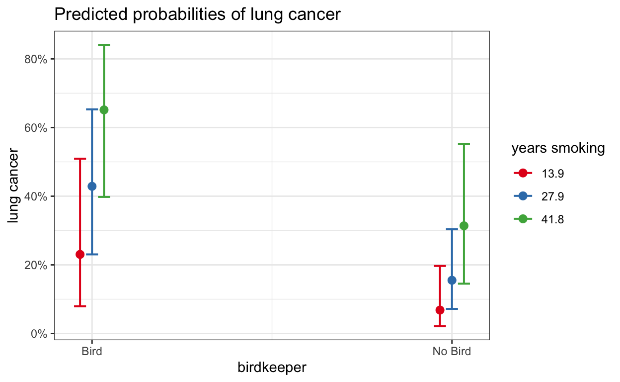
plot_model(glm_bk2, type = "pred", terms = c("birdkeeper", "years_smoking"))
# adding specific values
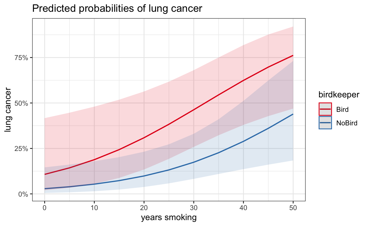
plot_model(glm_bk2, type = "pred", terms = c("years_smoking", "birdkeeper"))
This supplement was put together by Omar Wasow.