Topics and Concepts Covered
- Loading in data
- Cleaning data
- Working with dates
- Graphing data
Loading in Data
The data used in this handout comes from Roper’s iPoll database (https://ropercenter-cornell-edu.ezproxy.princeton.edu/). In order to create the data file, I went through iPoll and added about 30 polls about public approval of the Supreme Court to “My iPoll Folder.” Here is an example of the wording of one of the poll questions:
“Now, I’d like your opinion of some organizations and institutions. Is your overall opinion of the Supreme Court very favorable, mostly favorable, mostly unfavorable, or very unfavorable?”
I then went to the folder, selected all, and clicked “Download Toplines (csv)” on the right-hand side. This created a .csv file that I named “supreme_court_data.csv.” The first step is to load this data file into R.
# loading in data
court <- read.csv("supreme_court_data.csv", header = TRUE)

# checking data loaded properly
court %>% dplyr::glimpse()
Rows: 178
Columns: 17
$ QuestionID    <chr> "USPSRA.020906.R08FF2", "USPSRA.020906.R08FF2"…
$ RespTxt       <chr> "Very favorable", "Mostly favorable", "Mostly …
$ RespPct       <chr> "16", "44", "18", "10", "*", "12", "7", "56", …
$ QuestionTxt   <chr> "Now thinking about some groups and organizati…
$ QuestionNote  <chr> "* = less than .5%.", "* = less than .5%.", "*…
$ SubPopulation <chr> "Asked of Form 2 half sample", "Asked of Form …
$ ReleaseDate   <chr> "2/9/06", "2/9/06", "2/9/06", "2/9/06", "2/9/0…
$ SurveyOrg     <chr> "Princeton Survey Research Associates Internat…
$ SurveySponsor <chr> "Pew Research Center for the People & the Pres…
$ SourceDoc     <chr> "Pew News Interest Index Poll", "Pew News Inte…
$ BegDate       <chr> "2/1/06", "2/1/06", "2/1/06", "2/1/06", "2/1/0…
$ EndDate       <chr> "2/5/06", "2/5/06", "2/5/06", "2/5/06", "2/5/0…
$ ExactDates    <chr> "Y", "Y", "Y", "Y", "Y", "Y", "Y", "Y", "Y", "…
$ SampleDesc    <chr> "national adult", "national adult", "national …
$ SampleSize    <int> 1502, 1502, 1502, 1502, 1502, 1502, 2003, 2003…
$ IntMethod     <chr> "telephone", "telephone", "telephone", "teleph…
$ StudyNote     <chr> " ", " ", " ", " ", " ", " ", " ", " ", " ", "…
If your dataset isn’t too big, it’s also sometimes helpful to view
the full dataset. You can do this by clicking on the dataset in the
environment window on the right in R Studio, or with the
View() command in the console.
Cleaning Data
The next step is to clean this data so that it’s easier to work with.
# cleaning column names so that they're all lower case and one word
court <- court %>% janitor::clean_names()

# check names
court %>% colnames()
 [1] "question_id"    "resp_txt"       "resp_pct"
 [4] "question_txt"   "question_note"  "sub_population"
 [7] "release_date"   "survey_org"     "survey_sponsor"
[10] "source_doc"     "beg_date"       "end_date"
[13] "exact_dates"    "sample_desc"    "sample_size"
[16] "int_method" "study_note" Let’s rename and group the responses so that we can graph those who
favor or oppose the Supreme Court. I’m going to use the
case_when() command, which acts similarly to an
ifelse() or recode() statement but has more
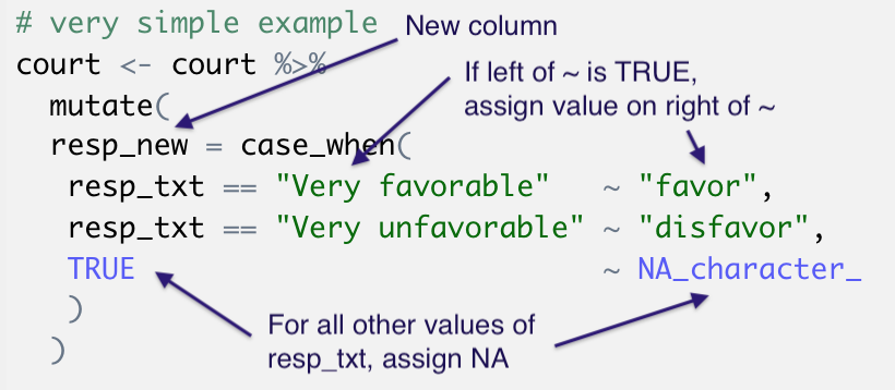
flexibility. Here’s a simple diagram explaining the structure of
case_when():

As with other kinds of logical statements, you can use symbols like
the vertical bar | to mean “or.” This allows multiple
responses to be coded as the same value. You can also use
& to set multiple limits on a variable. The tilde
~ separates the logical or if statement from the assigned
result. So a statement within the case_when() command which
reads
can be translated into english as “in the case when resp_txt
equals”Very favorable” or in the case when resp_txt equals “Mostly
favorable,” code “favor.” case_when() will recode variables
in order, so make sure you’re assigning values in a logical
progresion.
Similarly, we can recode text that has an ordered structure to be numeric with something like this:
# simple example converting ordered text response to numeric
court <- court %>%
  mutate(
  resp_num = case_when(
   resp_txt == "Very favorable"   ~ 1,
   resp_txt == "Favorable"        ~ 2,
   resp_txt == "No opinion"       ~ 3,
   resp_txt == "Unfavorable"      ~ 4,
   resp_txt == "Very unfavorable" ~ 5,
   TRUE                           ~ NA_real_ # anything not assigned gets NA
   )
  )
# more complex example sorting into favor and oppose
court <- court %>%
  dplyr::mutate(
    resp_new = case_when(

    resp_txt == "Very favorable" |
      resp_txt == "Mostly favorable" |
      resp_txt == "Favorable" |
      resp_txt == "Favorable strongly" |
      resp_txt == "Somewhat favorable" |
      resp_txt == "Favorable somewhat" ~ "favor", # make sure you don't forget a comma at
                                                  # the end of each assignment statement

    resp_txt == "Very unfavorable" |
      resp_txt == "Mostly unfavorable" |
      resp_txt == "Unfavorable" |
      resp_txt == "Unfavorable somewhat" |
      resp_txt == "Somewhat unfavorable" |
      resp_txt == "Unfavorable strongly" ~ "oppose",

    resp_txt == "Never heard of (Vol.)" |
      resp_txt == "Never heard of" ~ "never_heard",

    resp_txt == "Don't know/Not sure" |
      resp_txt == "Not sure" |
      resp_txt == "Undecided" |
      resp_txt == "No opinion" ~ "unsure",

    resp_txt == "Can't rate" |
      resp_txt == "Can't rate/Refused" |
      resp_txt == "Can't rate (Vol.)" |
      resp_txt == "Can't rate/Refused (Vol.)" |
      resp_txt == "Can't rate (Vol.)/Refused" |
      resp_txt == "Refused/Not answered" |
      resp_txt == "No answer" ~ "refused",

    TRUE ~ NA_character_ # I use a character form of NA because the rest of the recoded
                         # values are characters. If I was recoding to numbers I would use
                         # NA_integer instead. case_when() is very picky about this. When in
                         # doubt, try NA_real_.
  ),
  resp_pct = as.numeric(resp_pct) # recoding resp_pct to numeric. Notice this is a second
                                  # argument in the mutate command, not part of case_when()
)

# looking at number of observations in each category
# tidy version of table() command which allows you to use pipes

# original data
court %>% janitor::tabyl(resp_txt)
                  resp_txt  n percent
                            1 0.00562
                Can't rate  2 0.01124
         Can't rate (Vol.)  4 0.02247
 Can't rate (Vol.)/Refused 11 0.06180
        Can't rate/Refused  4 0.02247
 Can't rate/Refused (Vol.)  2 0.01124
       Don't know/Not sure  1 0.00562
                 Favorable  1 0.00562
        Favorable somewhat  1 0.00562
        Favorable strongly  1 0.00562
          Mostly favorable 26 0.14607
        Mostly unfavorable 26 0.14607
            Never heard of  4 0.02247
     Never heard of (Vol.) 19 0.10674
                 No answer  1 0.00562
                No opinion  2 0.01124
                  Not sure  3 0.01685
      Refused/Not answered  1 0.00562
        Somewhat favorable  3 0.01685
      Somewhat unfavorable  3 0.01685
                 Undecided  1 0.00562
               Unfavorable  1 0.00562
      Unfavorable somewhat  1 0.00562
      Unfavorable strongly  1 0.00562
            Very favorable 29 0.16292
Very unfavorable 29 0.16292 resp_new n percent valid_percent
favor 61 0.34270 0.3446
never_heard 23 0.12921 0.1299
oppose 61 0.34270 0.3446
refused 25 0.14045 0.1412
unsure 7 0.03933 0.0395
<NA> 1 0.00562 NAThe results are now condensed into two options: favor and oppose. I
also coded categories for three kinds of nonresponse so that we can
check if any of these have significant movement over the years. The
TRUE statement codes NA for any other responses that the
rest of the code doesn’t cover. Notice that since the
case_when() function is inside a mutate command, I first
call the variable I want to recode values for (resp_txt) and then use
the case_when command after an equal sign to set new values.
Working with Dates
Oftentimes you need to recode dates in order to work with them in R.
The package lubridate makes this process very easy.
  end_date
1   2/5/06
2   2/5/06
3   2/5/06
4   2/5/06
5   2/5/06
6   2/5/06
# change dates to month-day-year format
court <- court %>% mutate(
date = mdy(end_date)
)
# check that the date transformation worked
court %>% select(end_date, date) %>% head()
  end_date       date
1   2/5/06 2006-02-05
2   2/5/06 2006-02-05
3   2/5/06 2006-02-05
4   2/5/06 2006-02-05
5   2/5/06 2006-02-05
6   2/5/06 2006-02-05
Further documentation about functions contained in the lubridate package can be found here: https://www.rdocumentation.org/packages/lubridate/versions/1.7.4
Graphing Data
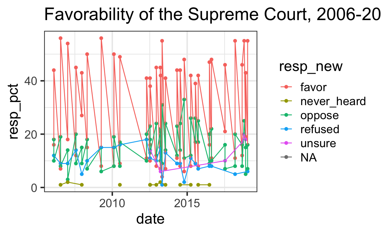
Lastly, let’s graph the data to see general trends in the perception of the Supreme Court.
# graph data
court %>%
  ggplot() +
    aes(x = date, y = resp_pct, color = resp_new) +
    geom_point() +
    geom_line() +
    ggtitle("Favorability of the Supreme Court, 2006-2019")

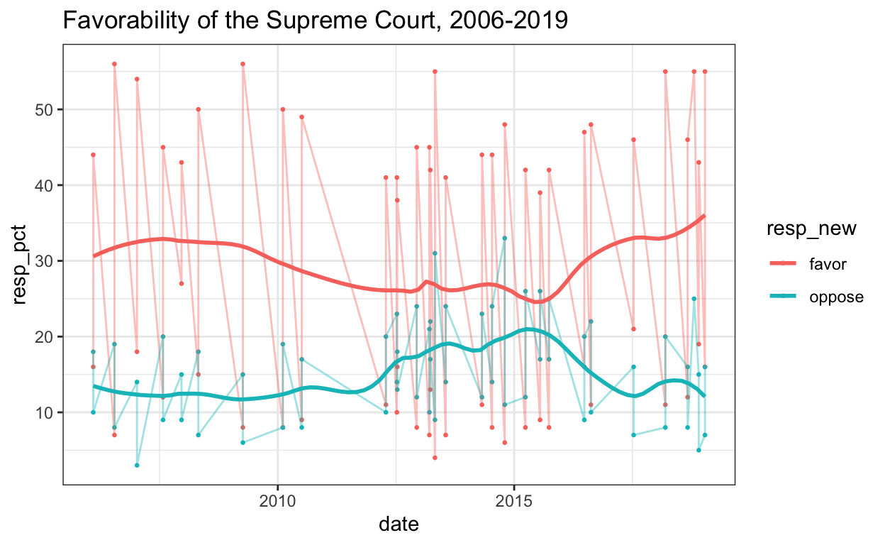
This graph is clearly too confusing to interpret. Let’s simplify to
only include “favor” and “oppose” results and add a smooth trend line to
show overall movement with
geom_smooth(span = .25, se = FALSE) (span
specifies the range of the running average and se controls
confidence intervals). Also, we’ll make the lines slightly transparent
using geom_line(alpha = .4) and shrink the size of the
points with geom_point(size = .5) to emphasize the smoothed
trend line. We’ll also add a black and white them with
theme_bw to remove the gray background. Finally, we’ll
assign the plot object to plot_out so we can modify it
easily later.
# graph data more simply
plot_out <- court %>%
  filter(resp_new == "favor" | resp_new == "oppose") %>%
  ggplot() +
    aes(x = date, y = resp_pct, color = resp_new) +
    geom_point(size  = .5) +
    geom_line(alpha  = .4) +
    geom_smooth(span = .25, se = FALSE) +
    ggtitle("Favorability of the Supreme Court, 2006-2019") +
    theme_bw()

plot_out

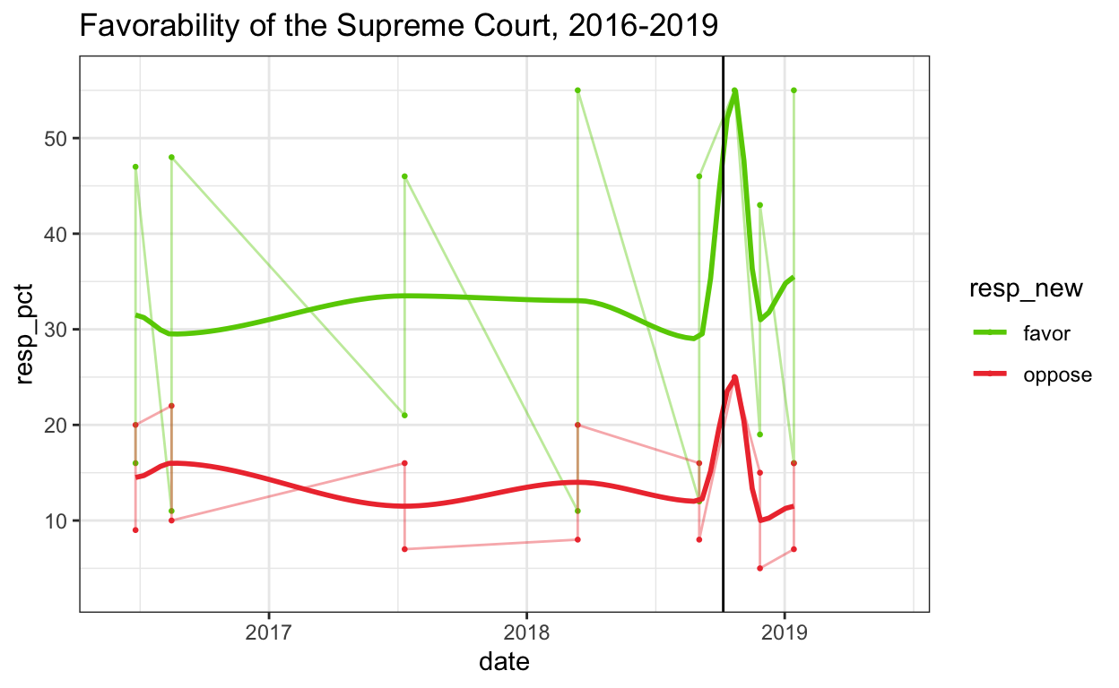
This is now a little easier to read. Lastly, let’s add a vertical line at Brett Kavanaugh’s nomination to see whether there was a change in favorability when he joined the Supreme Court. I’ll also add some x-axis limits to focus on the relevant time period and change the colors of the lines so that favor is green and oppose is red.
# graph data with vertical line
plot_out +
  # changing color of lines
  scale_colour_manual(values = c("chartreuse3", "brown2")) +
  # rescaling x axis
  xlim(as.Date("1/6/2016", "%d/%m/%Y"), as.Date("1/6/2019", "%d/%m/%Y")) +
  # vertical line
  geom_vline(xintercept = as.Date("6/10/2018", "%d/%m/%Y"), color = "black") +
  ggtitle("Favorability of the Supreme Court, 2016-2019")

There seems to be a rise in favorability at the time of Kavanaugh’s nomination, but without a statistical analysis of significance it is hard to say whether it’s just noise.
This supplement was put together by Risa Gelles-Watnick.