Background:
Governments across the developed and developing world often implement public policies seeking to improve the welfare of those citizens most in need. The WIC (Women, Infants and Children) program was designed to assist “low-income pregnant, breastfeeding, and non-breastfeeding postpartum women, and to infants and children up to age five who are found to be at nutritional risk.”1
How effective are these policies at improving social welfare? This is difficult to answer: first we must decide what are the relevant social indicators that we will measure. Second, there is the problem of confounding. Mothers and children who receive WIC will systematically differ from those who don’t. In particular, they will be on average poorer. So, for example, there may be dietary deficiencies that will affect the outcome of interest. How can we address that?
One approach would be to run randomized controlled trials (RCTs).
This raises ethical questions, however, about whether governments should
deliberately withhold benefits from citizens in the control group. An
alternative, given the absence of randomization, is matching. Through
matching, we try to achieve with observational data what randomization
aims to achieve by design: treatment and control groups that are
identical to one another except for the treatment assignment itself (on
average). To do so, we will use two packages: MatchIt and
cobalt.
install.packages("MatchIt")
install.packages("cobalt")
Here is a short working example with the car database
mtcars. Suppose we are interested in the relationship
between a “treatment,” vs, denoting the type of engine
(V-shaped or straight) and our outcome of interest, mpg,
miles-per-gallon. We are concerned, though, that there are systematic
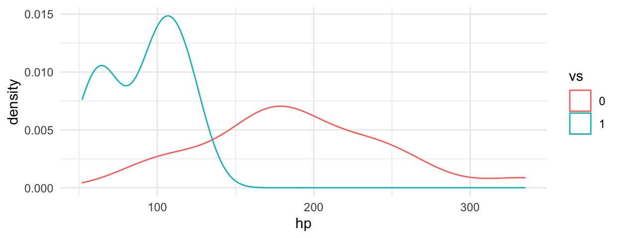
differences between the two vs types. For example, if we
compare the distribution of horsepower in the two types, we see
substantial areas of non-overlap:
To compare “apples to apples,” we want to find observations that are
similar on observed covariates. To do this, we match on other covariates
that we know will affect mpg: cyl,
hp and wt. We specify the treatment on the
left hand side (LHS), and the covariates we want to balance on the right
hand side (RHS): vs ~ cyl + hp + wt in the
formula argument.
Note that we specify method = "nearest" and
caliper = 0.1. These indicate that the algorithm will find
the nearest neighbors to our treatment observation, within a caliper
(tolerance parameter) of 0.1. Do not worry too much about it for now.2
mtcars_m_out <- matchit(
  formula = vs ~ cyl + hp + wt,
  data    = mtcars,
  method  = "nearest",
  caliper = 0.1
)
We then evaluate the matching process with commands like
summary(matchit_output). Looking at the output below, what
do you notice about the mean values for “treated” and “control” units in
all the data versus the matched data?
# overview of matching
mtcars_m_out
A matchit object
 - method: 1:1 nearest neighbor matching without replacement
 - distance: Propensity score [caliper]
             - estimated with logistic regression
 - caliper: <distance> (0.044)
 - number of obs.: 32 (original), 4 (matched)
 - target estimand: ATT
 - covariates: cyl, hp, wt
# more detailed summary
summary(mtcars_m_out)
Call:
matchit(formula = vs ~ cyl + hp + wt, data = mtcars, method = "nearest",
    caliper = 0.1)

Summary of Balance for All Data:
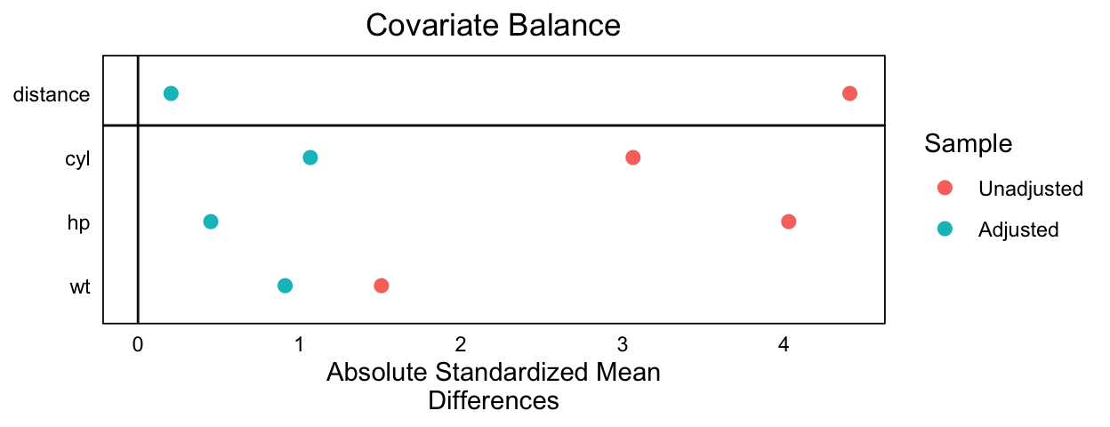
         Means Treated Means Control Std. Mean Diff. Var. Ratio
distance         0.867         0.104            4.41      0.526
cyl              4.571         7.444           -3.06      0.666
hp              91.357       189.722           -4.03      0.164
wt               2.611         3.689           -1.51      0.626
         eCDF Mean eCDF Max
distance     0.470    0.944
cyl          0.479    0.778
hp           0.385    0.833
wt           0.325    0.611


Summary of Balance for Matched Data:
         Means Treated Means Control Std. Mean Diff. Var. Ratio
distance         0.724         0.689           0.204      1.046
cyl              4.000         5.000          -1.067      0.000
hp              89.500       100.500          -0.450      6.119
wt               1.856         2.508          -0.910      0.874
         eCDF Mean eCDF Max Std. Pair Dist.
distance     0.129      0.5           0.204
cyl          0.167      0.5           1.067
hp           0.045      0.5           0.573
wt           0.172      0.5           0.994

Sample Sizes:
          Control Treated
All            18      14
Matched         2       2
Unmatched      16      12
Discarded       0       0
To convert the matchit object to a
data.frame, we use:
mtcars_match <- match.data(mtcars_m_out)
To check for covariate balance:
# abs = TRUE for absolute difference
cobalt::love.plot(mtcars_m_out, abs = TRUE)
Exercise
In this exercise, we will analyze a subset of white families from the ECLS (Early Childhood Longitudinal Study). We will focus on a set of family characteristics and the treatment, whether or not the child’s mother was a beneficiary of the WIC program. The outcome of interest is the student’s performance in reading and math tests at kindergarten.
Codebook:
wic: dummy variable, indicating whether or not child’s mother received WIC.age.k.fall: age of child fall of kindergarten yearbooks: number of books in homebooks.2: number of books squaredbirth.weight.lbs: child birth weight lbsbirth.weight.oz: child birth weight ozbirth.weight: total birth weight ozfemale: child is femalemath.irt.k.spring: student’s math grade in kindergarten.mother.age: mother agemother.at.least.30: binary variable for mother \(>=\) 30read.irt.k.spring: student’s reading grade in kindergarten.ses.comp: socioeconomic status compositeteenage.mother: binary variable for mother age \(<\) 20
# IMPORTANT: change chunk header above to eval = TRUE for knitting
library(dplyr)
library(ggplot2)
library(MatchIt)
library(cobalt)
library(stargazer)
library(kableExtra)
library(janitor)

# load data
ecls <- read.csv(url("http://appliedstats.org/data/ecls_white_small.csv")) %>%
  clean_names()

# treatment variable: convert to factor
ecls <- ecls %>%
  mutate(
    wic_fct = as.factor(wic)
  )

# change the style of ggplot output
theme_set(theme_minimal())
Questions:
- First, let’s get a sense of the “treatment” assignment. How many WIC beneficiaries are there?
ecls %>%
  count(wic_fct) %>%
  kable(
    caption = "Breakdown of beneficiaries of WIC",
    align   = "c"
  ) %>%
  kable_styling(position = "center")
| wic_fct | n |
|---|---|
| 0 | 5513 |
| 1 | 2129 |
Out of 7642 students, approximately two thousand have received the WIC.
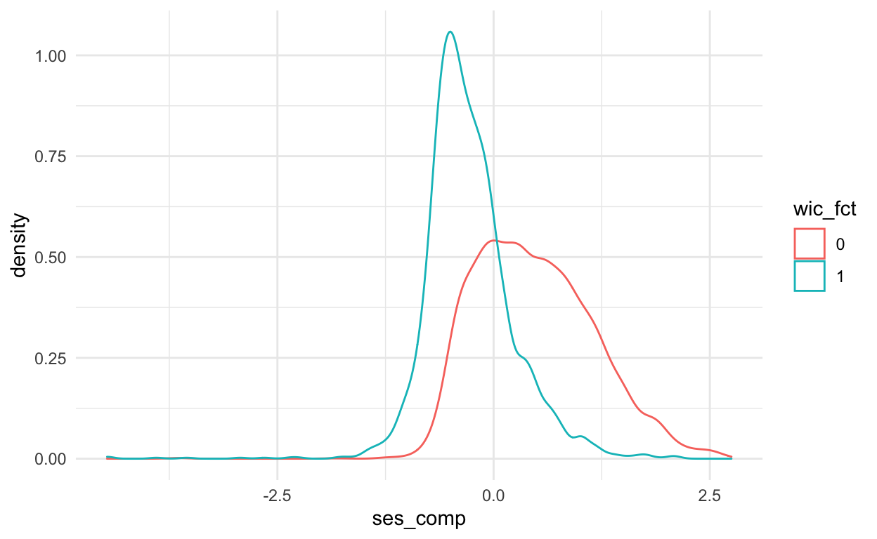
- The WIC program was targeted at poor families. Does the data reflect that? Create a density plot of socioeconomic status for beneficiaries and non-benefiaries. How would you interpret these graphs to an audience of non-statisticians?
# socioeconomic status
ecls %>%
  ggplot() +
  geom_density(
    aes(
      x     = ses_comp,
      group = wic_fct,
      col   = wic_fct
    )
  )
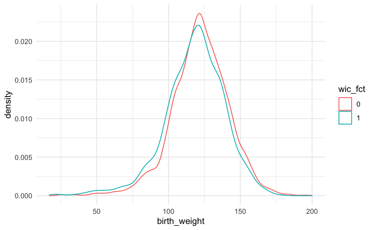
# child weight
ecls %>%
  ggplot() +
  geom_density(
    aes(
      x     = birth_weight,
      group = wic_fct,
      col   = wic_fct
    )
  )
- While have two outcomes of interest (student grades in reading and
math in kindergarten) for simplicity we’ll only focus on their reading
grades. Run a simple linear regression for the students’ reading grades
against their WIC recipient status. Additionally, run a separate model
with a full set of controls:
female,age_k_fall,ses_comp,books,books_2(books squared),birth_weight,mother_age. Display these models withstargazer, comparing the simple with the full model.
# baseline models
fit_read_base <- lm(read_irt_k_fall ~ wic, data = ecls)


# with controls
fit_read_control <- lm(
  read_irt_k_fall ~ wic + female + age_k_fall + ses_comp +
    books + books_2 + birth_weight + mother_age,
  data = ecls
)

stargazer(
  fit_read_base, fit_read_control,
  header = FALSE,
  type   = 'html'
)
| Dependent variable: | ||
| read_irt_k_fall | ||
| (1) | (2) | |
| wic | -4.810*** | -1.110*** |
| (0.219) | (0.241) | |
| female | 1.530*** | |
| (0.185) | ||
| age_k_fall | 0.427*** | |
| (0.021) | ||
| ses_comp | 2.810*** | |
| (0.156) | ||
| books | 0.039*** | |
| (0.007) | ||
| books_2 | -0.0001*** | |
| (0.00003) | ||
| birth_weight | 0.018*** | |
| (0.005) | ||
| mother_age | 0.223*** | |
| (0.021) | ||
| Constant | 25.900*** | -16.000*** |
| (0.116) | (1.750) | |
| Observations | 7,642 | 7,642 |
| R2 | 0.059 | 0.189 |
| Adjusted R2 | 0.059 | 0.188 |
| Residual Std. Error | 8.580 (df = 7640) | 7.970 (df = 7633) |
| F Statistic | 482.000*** (df = 1; 7640) | 222.000*** (df = 8; 7633) |
| Note: | p<0.1; p<0.05; p<0.01 | |
Interpret the results above. What is the relationship between student test scores and WIC? Can we make a causal claim? Why or why not?
To address concerns with confounding, let’s perform matching across treatment and control groups (WIC and non-WIC). Include all predictors of the model with controls. Make sure that the
caliperparameter is adjusted to0.1.
ecls_m_out <- matchit(
  formula = wic ~ female + age_k_fall + ses_comp +
    books + books_2 + birth_weight + mother_age,
  data    = ecls,
  method  = "nearest",
  caliper = 0.1
)

ecls_match <- match.data(ecls_m_out)
- Run
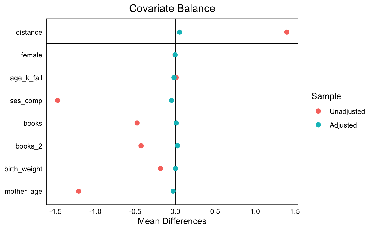
summary()on yourmatchitoutput. Look at the table under “Summary of balance for all data” and glance at the Means Treated and Means Control columns. Which covariates exhibit more balance (that is are similar in both treated and control conditions)? Are there covariates that seem far apart? Are some covariates already quite similar? Now look at the “Summary of balance for matched data.” Has there been improvement in balance?
summary(ecls_m_out)
Call:
matchit(formula = wic ~ female + age_k_fall + ses_comp + books +
    books_2 + birth_weight + mother_age, data = ecls, method = "nearest",
    caliper = 0.1)

Summary of Balance for All Data:
             Means Treated Means Control Std. Mean Diff. Var. Ratio
distance             0.523         0.184           1.399      1.504
female               0.488         0.491          -0.007          .
age_k_fall          68.879        68.834           0.011      0.986
ses_comp            -0.279         0.475          -1.474      0.562
books               77.629       104.201          -0.479      0.892
books_2           9099.551     14303.596          -0.429      0.711
birth_weight       118.052       121.962          -0.185      1.127
mother_age          21.500        26.676          -1.211      0.766
             eCDF Mean eCDF Max
distance         0.357    0.559
female           0.003    0.003
age_k_fall       0.004    0.013
ses_comp         0.187    0.495
books            0.120    0.224
books_2          0.120    0.224
birth_weight     0.024    0.073
mother_age       0.152    0.479


Summary of Balance for Matched Data:
             Means Treated Means Control Std. Mean Diff. Var. Ratio
distance             0.431         0.418           0.054      1.099
female               0.488         0.489          -0.003          .
age_k_fall          68.864        68.933          -0.016      0.973
ses_comp            -0.148        -0.124          -0.047      1.291
books               86.029        85.326           0.013      1.068
books_2          10636.470     10311.464           0.027      1.049
birth_weight       120.100       120.017           0.004      1.042
mother_age          22.591        22.711          -0.028      1.175
             eCDF Mean eCDF Max Std. Pair Dist.
distance         0.009    0.053           0.054
female           0.001    0.001           1.011
age_k_fall       0.005    0.017           1.141
ses_comp         0.011    0.075           0.586
books            0.011    0.024           1.040
books_2          0.011    0.024           0.990
birth_weight     0.005    0.022           1.075
mother_age       0.012    0.054           0.790

Sample Sizes:
          Control Treated
All          5513    2129
Matched      1563    1563
Unmatched    3950     566
Discarded 0 0- Display the covariate balance plot using
cobalt::love.plot()(see sample code above). Has the balance improved as a result of matching?
bal.tab(ecls_m_out)
Call
 matchit(formula = wic ~ female + age_k_fall + ses_comp + books +
    books_2 + birth_weight + mother_age, data = ecls, method = "nearest",
    caliper = 0.1)

Balance Measures
                 Type Diff.Adj
distance     Distance    0.054
female         Binary   -0.001
age_k_fall    Contin.   -0.016
ses_comp      Contin.   -0.047
books         Contin.    0.013
books_2       Contin.    0.027
birth_weight  Contin.    0.004
mother_age    Contin.   -0.028

Sample sizes
          Control Treated
All          5513    2129
Matched      1563    1563
Unmatched 3950 566love.plot(ecls_m_out)
- Re-run the analysis in (3). What differences do you note between these results and the ones you found before?
In unmatched data, the magnitude of our coefficient in the naive model is substantially larger than the coefficient in the model with controls suggesting that our estimate is driven non-trivially by the model we pick.
Notice, in the matched data, that moving from the naive model to the full model does not result in substantial changes in the magnitude of the estimate suggesting that our estimate is not model dependent.
# baseline models
fit_read_base_m <- lm(read_irt_k_fall ~ wic, data = ecls_match)

# with controls
fit_read_control_m <- lm(
  read_irt_k_fall ~ wic + female + age_k_fall + ses_comp +
    books + books_2 + birth_weight + mother_age,
  data = ecls_match
)


stargazer(
  fit_read_base_m, fit_read_control_m,
  type   = 'html',
  header = FALSE
)
| Dependent variable: | ||
| read_irt_k_fall | ||
| (1) | (2) | |
| wic | -1.320*** | -1.180*** |
| (0.267) | (0.254) | |
| female | 1.610*** | |
| (0.257) | ||
| age_k_fall | 0.347*** | |
| (0.030) | ||
| ses_comp | 2.310*** | |
| (0.271) | ||
| books | 0.058*** | |
| (0.009) | ||
| books_2 | -0.0002*** | |
| (0.00004) | ||
| birth_weight | 0.013** | |
| (0.006) | ||
| mother_age | 0.193*** | |
| (0.031) | ||
| Constant | 23.000*** | -9.890*** |
| (0.189) | (2.420) | |
| Observations | 3,126 | 3,126 |
| R2 | 0.008 | 0.105 |
| Adjusted R2 | 0.007 | 0.103 |
| Residual Std. Error | 7.470 (df = 3124) | 7.100 (df = 3117) |
| F Statistic | 24.300*** (df = 1; 3124) | 45.800*** (df = 8; 3117) |
| Note: | p<0.1; p<0.05; p<0.01 | |
As further evidence that our estimate with the matched data is less
model dependent (e.g., results determined by how we specify the model
with controls, interactions, quadratics, etc.), here is a contrast of
t.test() results with the unmatched and then the matched
data. The t.test with matched data produces similar
estimates to both the naive and the full regression models with matched
data.
t.test(read_irt_k_fall ~ wic, data = ecls) %>%
  broom::tidy() %>%
  select(contains("estimate"),statistic, p.value, contains("conf")) %>%
  kable(format = "html", digits = 2) %>%
  kable_styling(bootstrap_options = "striped", full_width = FALSE)
| estimate | estimate1 | estimate2 | statistic | p.value | conf.low | conf.high |
|---|---|---|---|---|---|---|
| 4.81 | 25.9 | 21.1 | 24.7 | 0 | 4.43 | 5.19 |
t.test(read_irt_k_fall ~ wic, data = ecls_match) %>%
  broom::tidy() %>%
  select(contains("estimate"),statistic, p.value, contains("conf")) %>%
  kable(format = "html", digits = 2) %>%
  kable_styling(bootstrap_options = "striped", full_width = FALSE)
| estimate | estimate1 | estimate2 | statistic | p.value | conf.low | conf.high |
|---|---|---|---|---|---|---|
| 1.32 | 23 | 21.7 | 4.93 | 0 | 0.79 | 1.84 |
Given this analysis, what would you recommend to a policy-maker? Should we continue the WIC program or should we think about redesigning it? There is no “right” answer, use your critical thinking and use the statistical evidence to inform your opinion.
What are some limitations of matching we should keep in mind?
Questions
- Regression vs Matching:
- Why isn’t regression enough to control for imbalance? First, we want to focus analysis on the area of common support (the subset of our data in which there is overlap between treated and control subjects). For example, including rich people in an analysis of anti-poverty programs is probably not meaningful as they would be “never takers” of the benefit. Another related idea is that in any data analysis we can have outliers for which there is no “twin” subject but which could exert significant influence on results. Regression will not address either of these issues and will just find the line that fits the data. Matching, on the other hand, has the potential to focus our analysis on the observations that could plausibly be either “treated” or “control” (area of common support) and prunes the extreme or outlying observations for which there aren’t meaningful comparisons or “twins.”
- Model dependence:
- Why didn’t the results didn’t change much between matched and
unmatched regression? If results do not change much between unmatched
and matched subsets, that suggests the estimated relationships are not
being driven by imbalance in data. Put another way, matching can be seen
as a kind of robustness check to see whether the results are sensitive
to imbalance. In the WIC example above, adding controls shrunk the
magnitude of the coefficient a lot between the naive and the “full”
models suggesting that in the naive model, WIC is correlated with a lot
of other covariates and the results are sensitive to the model. In the
matched data, though, the coefficient on the naive model and the full
model are quite similar. This shows us that matching has reduced model
dependence. Just for comparison, we can see that a simple
t.test()gives us a similar estimate to the full model, suggesting matching has reduced model dependence.
- Why didn’t the results didn’t change much between matched and
unmatched regression? If results do not change much between unmatched
and matched subsets, that suggests the estimated relationships are not
being driven by imbalance in data. Put another way, matching can be seen
as a kind of robustness check to see whether the results are sensitive
to imbalance. In the WIC example above, adding controls shrunk the
magnitude of the coefficient a lot between the naive and the “full”
models suggesting that in the naive model, WIC is correlated with a lot
of other covariates and the results are sensitive to the model. In the
matched data, though, the coefficient on the naive model and the full
model are quite similar. This shows us that matching has reduced model
dependence. Just for comparison, we can see that a simple
- Causality:
- Can we make causal claims? In general, no. While matching helps approximate experimental designs to make a causal claim we have to make assumptions that are often assumed to be heroic. In particular, we have to assume that matching on observed characteristics also results in matching on unobserved characteristics (e.g., unmeasured).
For more information, see https://www.fns.usda.gov/wic/women-infants-and-children-wic ↩︎
But if you really do, you can read this excellent Wikipedia article on matching through propensity score (here)[https://en.wikipedia.org/wiki/Propensity_score_matching].↩︎
