Topics and Concepts Covered
- Permutation Tests
- The Rank Sum Test
Space Shuttle O-Ring Failures
In this example, researchers hypothesize that colder temperatures are associated with fuel seal problems and O-Ring failures.
We begin by reading in the data and viewing a bit of it.
# Uncomment lines below to install packages
# install.packages("Sleuth2")
# install.packages("ggplot2")
# install.packages("janitor")

# Loading required libraries
library(Sleuth2)
library(ggplot2)
library(janitor)

# Reading data
space <- Sleuth2::case0401

# Cleaning and viewing data
space <- janitor::clean_names(space)
head(space)
  incidents launch
1         1   Cool
2         1   Cool
3         1   Cool
4         3   Cool
5         0   Warm
6         0   Warm
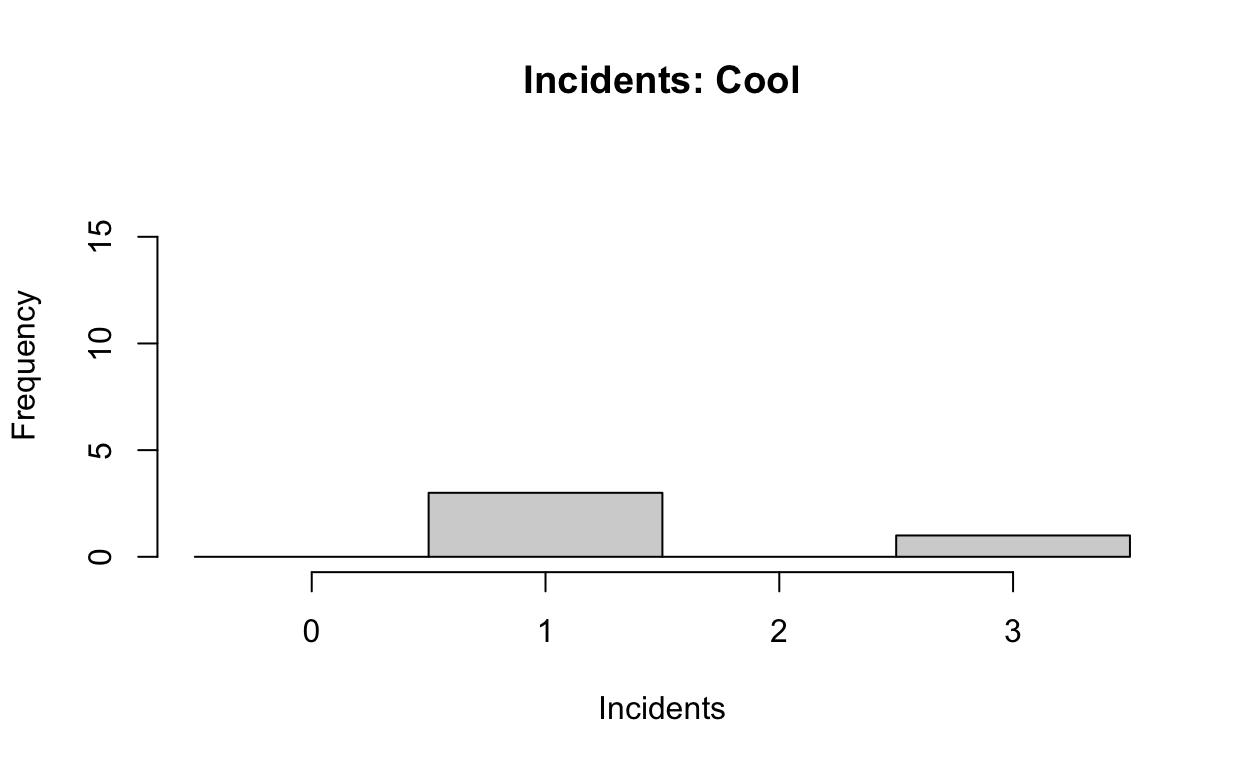
The data are 24 readings. Each reading has either a Cool or a Warm temperature at launch, and is associated with the number of incidents recorded.
We can visualise this data using a histogram.
his1 <- hist(space$incidents[space$launch=="Cool"],
             main = "Incidents: Cool",
             xlab = "Incidents",
             breaks = seq(-0.5,3.5),
             ylim=c(0,18) )
his2 <- hist(space$incidents[space$launch=="Warm"],
             main = "Incidents: Warm",
             xlab = "Incidents",
             breaks = seq(-0.5,3.5),
             ylim = c(0,18) )
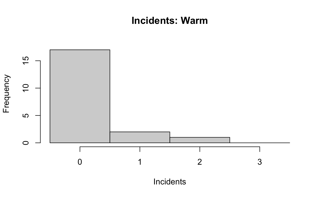
Note: type hist into the R help window for a full list
of parameters you can adjust. For instance, the ylim
parameter that allows us to keep y-axis scaled equivalently across
graphs for better comparison of data.
Alternately, we can try looking at the data using
ggplot
space %>%
  ggplot() +
    aes(x=incidents) +
    geom_histogram(binwidth = 1) +
    xlim(-0.5,4.5) +
    facet_grid( ~ launch) +
    labs(title="Distribution of Incidents by Launch Weather")
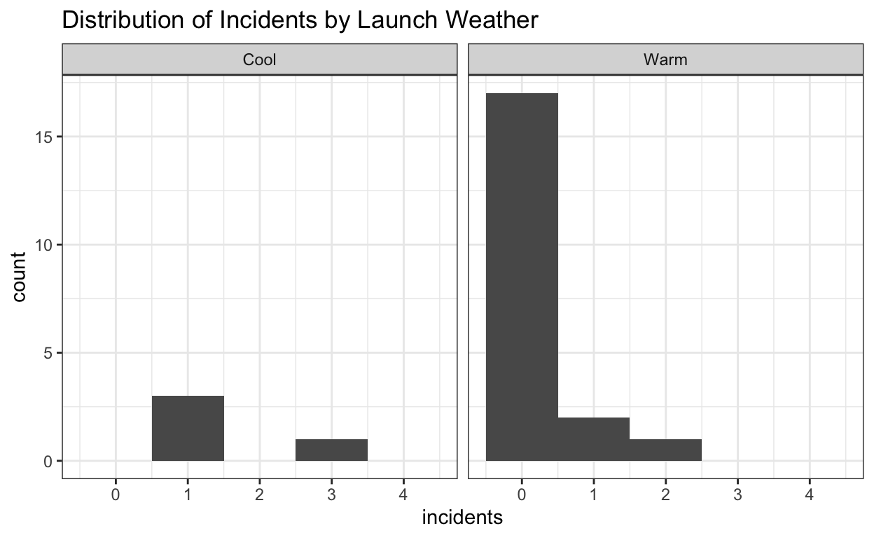
Here, a simple \(t\)-test is unable to be of much use because the distributions are so non-normal, and conventional transformations like taking the log are not helpful. Instead, we can use a Permutation Test to see how extreme our observed data are.
Permutation Test
As noted above, the data on O-ring incidents violates the assumption of normality so we should not use a conventional \(t\)-test.
A permutation test does not assume the data follow any distribution and, therefore, is appropriate for analyzing this data. A permutation test finds a \(p\)-value as the proportion of regroupings of the data that lead to test statistics at least as extreme as the observed one.
We first choose a test statistic, such as a difference in averages or a \(t\)-statistic, and then see how many regroupings of the data provide a test statistic as extreme as our observed case.
The total number of regroupings would be the number of ways to choose 4 terms in a group out of 24 terms. This is expressed as \(C_{24,4}\) and is articulated as “24 choose 4”.
\[ C_{n,r} = \binom{n}{r} = \frac{n!}{r!(n-r)!} \]
[1] 10626And so, there are 10,626 ways of regrouping 24 observations into groups where \(n_1\) = 4, and \(n_2\) = 20.
Since there are 17 zeros, 5 ones, 1 two, and 1 three, these are the only 16 possible unique combinations possible:
- (0, 0, 0, 0)
- (0, 0, 0, 1)
- (0, 0, 0, 2)
- (0, 0, 0, 3)
- (0, 0, 1, 1)
- (0, 0, 1, 2)
- (0, 0, 1, 3)
- (0, 0, 2, 3)
- (0, 1, 1, 1)
- (0, 1, 1, 2)
- (0, 1, 1, 3)
- (0, 1, 2, 3)
- (1, 1, 1, 1)
- (1, 1, 1, 2)
- (1, 1, 1, 3)
- (1, 1, 2, 3)
Our observed outcome was (1, 1, 1, 3). We should see which outcomes give us \(t\)-statistics that are as or more extreme as our observed case. It turns out, the only cases are: (1, 1, 2, 3) and (0, 1, 2, 3).
# t.test for (1, 1, 2, 3), i.e, observations 1, 2, 4 and 24

# Checking observations
space$incidents[c(1, 2, 4, 24)]
[1] 1 1 3 2# Running t-test
t.test(space$incidents[c(1, 2, 4, 24)],
space$incidents[-c(1, 2, 4, 24)],
var.equal = TRUE)
    Two Sample t-test

data:  space$incidents[c(1, 2, 4, 24)] and space$incidents[-c(1, 2, 4, 24)]
t = 6, df = 22, p-value = 5e-06
alternative hypothesis: true difference in means is not equal to 0
95 percent confidence interval:
 1.04 2.16
sample estimates:
mean of x mean of y
     1.75      0.15
Here, the \(t\)-statistic is 5.95. Similarly, we compute the \(t\)-statistic for the case (0, 1, 2, 3).
# t.test for (0, 1, 2, 3), i.e, observations 1, 4, 5 and 24

# Checking observations
space$incidents[c(1, 4, 5, 24)]
[1] 1 3 0 2# Running t-test
t.test(space$incidents[c(1, 4, 5, 24)],
space$incidents[-c(1, 4, 5, 24)],
var.equal = TRUE)
    Two Sample t-test

data:  space$incidents[c(1, 4, 5, 24)] and space$incidents[-c(1, 4, 5, 24)]
t = 4, df = 22, p-value = 8e-04
alternative hypothesis: true difference in means is not equal to 0
95 percent confidence interval:
 0.607 1.993
sample estimates:
mean of x mean of y
      1.5       0.2
Here the \(t\)-statistic is also 3.888.
Given that there are 10626 ways of regrouping all 24 terms. We need to know how many ways there are to choose the three groups with \(t\)-statistics as or more extreme as our observed \(t\)-statistic. i.e. we need to calculate how many different ways we can create groups of (1, 1, 1, 3), (1, 1, 2, 3), and (0, 1, 2, 3).
For (1, 1, 1, 3), we have to choose 3 ones out of five [\(C_{5,3}\)] and we have to choose the one three observed [\(C_{1,1}\)].
And so, \(C_{1,1,1,3} = C_{5,3}* C_{1,1}\)
[1] 10And, \(C_{1,1,2,3} = C_{5,2}* C_{1,1}* C_{1,1}\)
And, \(C_{0,1,2,3} = C_{17,1}* C_{5,1}* C_{1,1}* C_{1,1}\)
c0123 <- 17* 5* 1* 1
c0123
[1] 85Now we calculate the \(p\)-value as a probability of observing such an extreme \(t\)-statistic against all possible regroupings.
p <- (c1113 + c1123 + c0123)/c24.4
p
[1] 0.00988We calculate the \(p\)-value to be approximately 0.01.
We can also estimate the \(p\)-value by sampling a subset of all possible permutations.
# Finding number of rows of data
num_rows <- nrow(space)
num_rows
[1] 24# Finding observed difference in means
obs_diff_in_means <- mean(space$incidents[space$launch=="Cool"]) - mean(space$incidents[space$launch=="Warm"])
obs_diff_in_means
[1] 1.3# If we randomly assign "treatment" and "control" (or warm and cool), what is the difference in means?
rand_diff_in_means <- NA
randomizations <- 1000
for (i in 1:randomizations) {
regrouped <- sample(space$incidents, replace = FALSE) # randomly reshuffle without replacement
group1 <- regrouped[1:4]
group2 <- regrouped[5:num_rows]
rand_diff_in_means[i] <- mean(group1) - mean(group2)
}
# How extreme is our observed difference in means compared with distribution of randomization distribution
hist(rand_diff_in_means)
abline(v = obs_diff_in_means,
col = "red")
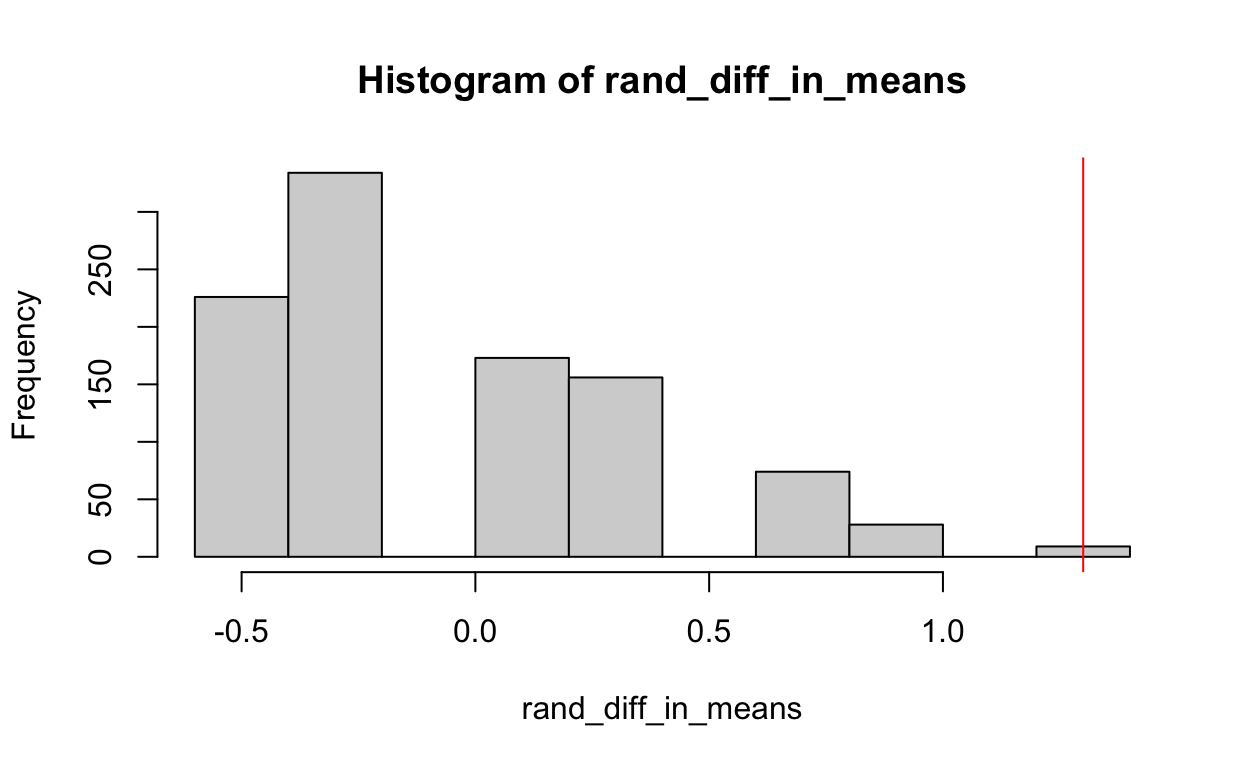
# What percent of our randomized difference in means are as or more extreme than observed difference
sum(rand_diff_in_means >= obs_diff_in_means) / randomizations
[1] 0.009Cognitive Load Theory in Teaching
In case 4.2 in Sleuth, researchers ask whether using modified instructional material results in quicker problem solving.
In this experiment of 28 subjects, 14 students were assigned the modified material, and 14 were assigned the conventional material.
We begin by reading in and summarizing the data.
# Reading data
teaching <- Sleuth2::case0402 %>% clean_names()

head(teaching)
  time  treatmt censor
1   68 Modified      0
2   70 Modified      0
3   73 Modified      0
4   75 Modified      0
5   77 Modified      0
6   80 Modified      0
# ggplot
ggplot(data = teaching) +
aes(x = treatmt,
y = time) +
geom_boxplot() +
ggtitle("Boxplot of solving time")
ggplot(data = teaching) +
  aes(x = time,
      color = treatmt) +
  geom_density() +
  scale_x_continuous(limit = c(0,400)) +
  ggtitle("Density plot of solving time")
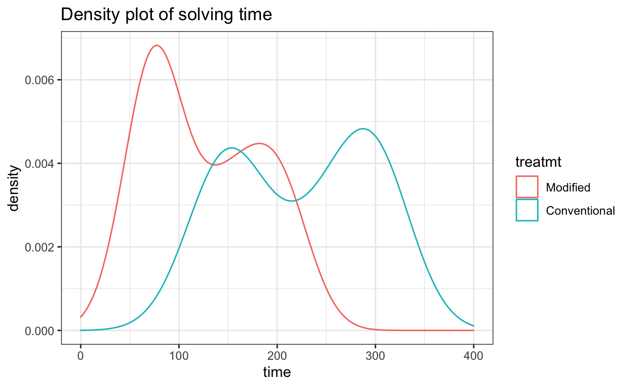
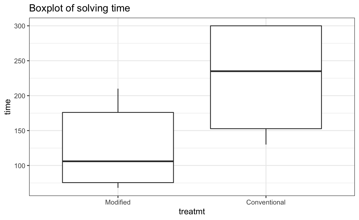
It appears that for modified instruction group, solution times are lower, but the distributions are extremely skewed – especially since the conventional group included five students who were not able to answer certain questions within the 300 second window.
Here, instead of doing a two-sample \(t\)-test, we can use a more resistant alternative: the Rank-Sum Test.
The Rank-Sum Test
The Rank-Sum test is more resistant to outliers because it transforms the data by simply ranking each measure in the combined sample, thus eliminating the need for population distributions altogether. This feature makes it attractive for situations of censored observations, i.e. when there is a hard cutoff in the recording of data, like students who took more than 300 seconds to answer were censored.
The Rank Sum test first ranks all measurements in increasing order. Any ties are split evenly – e.g. if the 6th and 7th observations both have the same score, then they both receive the rank of 6.5 [i.e. the average of the orders].
rank <- rank(teaching$time, ties.method = "average")
rank
 [1]  1.0  2.0  3.0  4.0  5.0  6.5  6.5  9.0 12.0 14.0 17.0 18.0 19.0
[14] 20.0  8.0 10.0 11.0 13.0 15.0 16.0 21.0 22.0 23.0 26.0 26.0 26.0
[27] 26.0 26.0
We then sum the ranks for all students of a particular group. Here, we sum the ranks of all students in the modified instructional group. This will be our test statistic, \(T\).
t_m <- sum(rank[teaching$treatmt == "Modified"])
t_m
[1] 137We observe \(t_m\) as the Test statistic for the Modified group. We need to see whether this test statistic is extreme. And so we assume that these \(T\)-statistics are normally distributed. To implement our assumption, we need to build a normal distribution of test statistics.
ave <- mean(rank)
ave
[1] 14.5sd <- sd(rank)
sd
[1] 8.2# n_m gives the number of observations in group Modified.
n_m <- nrow(subset(teaching, teaching$treatmt == "Modified"))
n_m
[1] 14#For a normal distribution of T statistics, we need a mean t and its standard deviation.
mean_t <- n_m * ave
mean_t
[1] 203sd_t <- sd * sqrt((n_m^2)/(2* n_m))
sd_t
[1] 21.7And so now that we have a normal distribution of \(T\)-statistics, we can calculate the \(z\)-score, and thus the \(p\)-value of observing our initial \(T\)-statistic of 137.
And so, the one sided $$-value is 0.001.
We can also just use the Wilcoxon Rank-Sum Test function in
R.
wilcox.test(time ~ treatmt,
            conf.int = TRUE,
            exact = TRUE,
            data = teaching)
    Wilcoxon rank sum test with continuity correction

data:  time by treatmt
W = 32, p-value = 0.003
alternative hypothesis: true location shift is not equal to 0
95 percent confidence interval:
 -160  -57
sample estimates:
difference in location
                   -94
By this method, we see a \(p\)-value
of 0.00254. We can adjust the parameters of the wilcox test to give us a
one sided \(p\)-value by including the
parameter alternative = "greater". Note: we have previously
used this modification in the Welch’s \(t\)-test function.
wilcox.test(time ~ treatmt,
            conf.int = TRUE,
            alternative = "greater",
            exact = TRUE,
            data = teaching)
    Wilcoxon rank sum test with continuity correction

data:  time by treatmt
W = 32, p-value = 1
alternative hypothesis: true location shift is greater than 0
95 percent confidence interval:
 -152  Inf
sample estimates:
difference in location
                   -94