Introduction
Imagine if we were interested in how attitudes about civil unrest in the 1970s influenced political views. To investigate, we could use the American National Election Study Timeseries to model and plot how something like the relationship between the 1972 Unrest Scale relates to feelings toward the Republican presidential candidate.
Load data
anes <- haven::read_dta("anes_timeseries_cdf_dta/anes_timeseries_cdf_stata13.dta")
NOTE: The haven package has a useful feature when
importing the formats .dta or .sav which is
that it keeps each columns label information that is stored with those
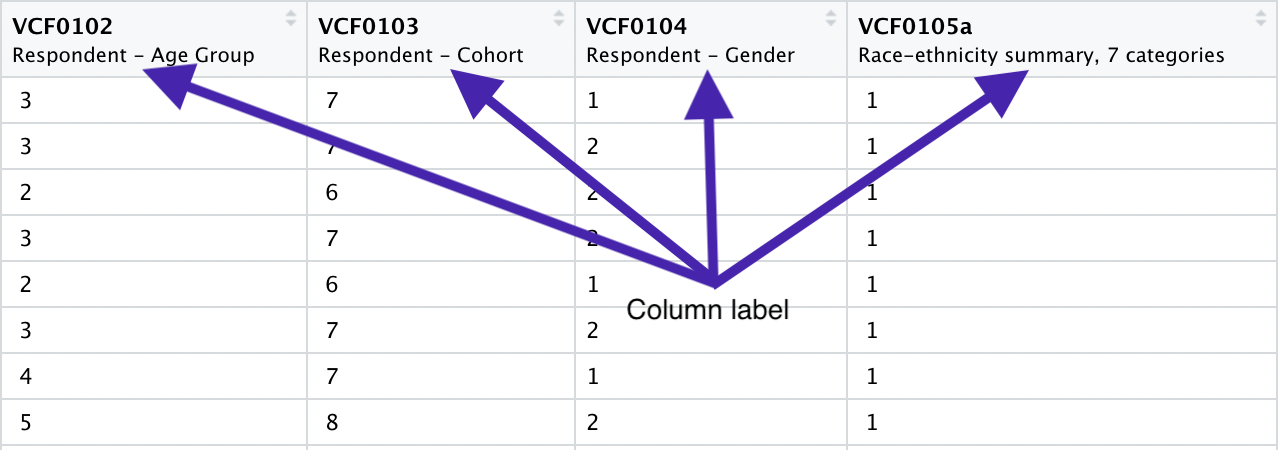
data. For example we might look at the variable V201600 and
we can see the @ label that tells us the question description. This is
called metadata (data about our data). We can also see that the type of
data is dbl+lbl. This is short for double — typical of
numeric data that’s not integers — and label.

Identify
column label with sjlabelled::get_label (without S)
# get column label with `get_label` (NO S)
sjlabelled::get_label(anes$VCF0104)  # sex
[1] "Respondent - Gender"sjlabelled::get_label(anes$VCF0426) # thermometer GOP candidate
[1] "Thermometer - Republican Presidential Candidate"Identify
meaning of responses with sjlabelled::get_labels (with
S)
# get column label with `get_label`
sjlabelled::get_label(anes$VCF0105a)
[1] "Race-ethnicity summary, 7 categories"So we know anes$VCF0105a is a measure of self-reported
race but it can still be hard to know what the responses mean. For
example, what does race = 5 mean?
table(anes$VCF0105a)
    1     2     3     4     5     6     7
46035  6906   565   340  3942   561    55
The codebook will have answers but we can also use
sjlabelled::get_labels (with an S) to learn how the numbers
map to categories (in this case race).
# get explanation of responses with `get_labels` (WITH S)
sjlabelled::get_labels(anes$VCF0105a)
[1] "1. White non-Hispanic (1948-2012)"
[2] "2. Black non-Hispanic (1948-2012)"
[3] "3. Asian or Pacific Islander, non-Hispanic (1966-2012)"
[4] "4. American Indian or Alaska Native non-Hispanic (1966-2012)"
[5] "5. Hispanic (1966-2012)"
[6] "6. Other or multiple races, non-Hispanic (1968-2012)"
[7] "7. Non-white and non-black (1948-1964)"
[8] "9. Missing"
Recode data
anes <- anes %>%
  mutate(
    # this is a time series version of ANES with multiple years
    year       = VCF0004 %>% as.factor(),

    # create column for age
    age        = VCF0102 %>% as.numeric(),

    # convert sex to binary
    male_bin   = case_when(
                   VCF0104 == 1 ~ 1,
                   TRUE         ~ 0) %>% as.numeric(),

    # convert sex to factor
    male_fct   = case_when(
                   VCF0104 == 1 ~ "Male",
                   VCF0104 == 2 ~ "Female"
                  ) %>% as.factor(),

    # create race numeric
    race_num   = VCF0105a %>% as.numeric(),

    # create race factor
    race_fct   = case_when(
      VCF0105a == 1 ~ "White",
      VCF0105a == 2 ~ "Black",
      VCF0105a == 3 ~ "AAPI",
      VCF0105a == 4 ~ "Native American",
      VCF0105a == 5 ~ "Hispanic",
      VCF0105a == 6 ~ "Other",
      VCF0105a == 7 ~ "Other", # combine two categories
      VCF0105a == 9 ~ NA_character_
    ) %>% as.factor(),

    # create smaller race factor
    race5_fct   = case_when(
      VCF0105a == 1 ~ "White",
      VCF0105a == 2 ~ "Black",
      VCF0105a == 3 ~ "AAPI",
      VCF0105a == 5 ~ "Hispanic",
      TRUE          ~ "Other"
    ) %>% as.factor(),

    # example: variable with just Whites and Blacks
    race_wb_fct    = case_when(
                       race_num == 1 ~ "White",
                       race_num == 2 ~ "Black",
                       TRUE      ~ NA_character_
                       ) %>% as.factor(),

    # example: create race dummy (0/1) variables
    race_white_bin  = ifelse(race_num == 1, 1, 0) %>% as.numeric(),
    race_black_bin  = ifelse(race_num == 2, 1, 0) %>% as.numeric(),
    race_aapi_bin   = ifelse(race_num == 3, 1, 0) %>% as.numeric(),
    race_native_bin = ifelse(race_num == 4, 1, 0) %>% as.numeric(),
    race_hisp_bin   = ifelse(race_num == 5, 1, 0) %>% as.numeric(),
    race_other_bin  = ifelse(race_num == 6 &
                             race_num == 7, 0, 1) %>% as.numeric(),

    # main explanatory and outcome vars
    unrest_scale   = VCF0528 %>% as.numeric(),
    therm_rep_pres = VCF0426 %>% as.numeric()
  )
Remove label info
Once we’ve finished scrubbing the data, it’s helpful to clean labels
because many R functions have difficulty with labeled
data.
For example, lm() works just fine with labeled data.
sjPlot::plot_model() however will break on labeled
data.
# in general DO NOT use raw variables you haven't recoded as they'll include values like 998 for missing data

# example: this works
lm1 <- lm(VCF0426 ~ VCF0104, data = a72)

# example: this generates an error due to labeled data
sjPlot::plot_model(lm1, type = "pred", terms = "VCF0104")

# Error: Can't combine `..1` <character> and `..2` <double>.
# Run `rlang::last_error()` to see where the error occurred.
One method is to recode individual variables while scrubbing with
commands like as.numeric() or as.character()
or as.factor(). See sample code below:
anes <- anes %>%
  mutate(
    feel_trump = VCF9057 %>% as.numeric(),

    male_fct   = case_when(
      VCF0104 == 1 ~ "Male",
      VCF0104 == 2 ~ "Female",
    ) %>% as.factor()
  )

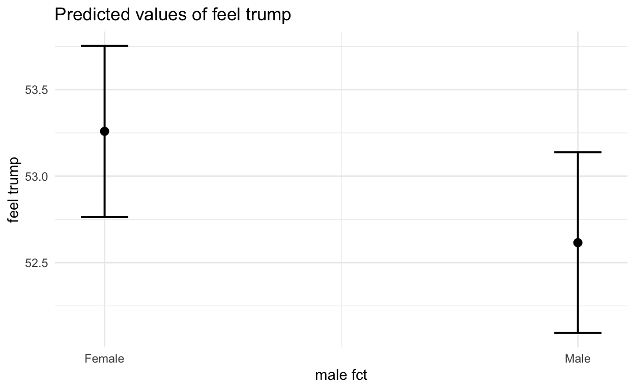
# Now, sjPlot::plot_model() works
lm1 <- lm(feel_trump ~ male_fct, data = anes)
sjPlot::plot_model(lm1, type = "pred", terms = "male_fct")

Remove all labels
zap_labels
Another method is to zap all labels:
# remove all label info from data
# NOTE: ignore Warning messages
anes <- sjlabelled::zap_labels(anes)
Model data
Typically we might control for something like 5-7 variables. In this example, we just use a handful to illustrate.
Run two models: bivariate and multiple terms
# Thermometers Republican Candidate vs Unrest Scale
reduced_model <- lm(formula = therm_rep_pres ~ unrest_scale,
          data    = a72)

summary(reduced_model)
Call:
lm(formula = therm_rep_pres ~ unrest_scale, data = a72)

Residuals:
   Min     1Q Median     3Q    Max
-68.20 -14.75   5.25  20.25  34.56

Coefficients:
             Estimate Std. Error t value Pr(>|t|)
(Intercept)     61.29       2.28   26.93   <2e-16 ***
unrest_scale     1.15       0.67    1.72    0.086 .
---
Signif. codes:  0 '***' 0.001 '**' 0.01 '*' 0.05 '.' 0.1 ' ' 1

Residual standard error: 26.4 on 732 degrees of freedom
  (1971 observations deleted due to missingness)
Multiple R-squared:  0.00402,   Adjusted R-squared:  0.00266
F-statistic: 2.95 on 1 and 732 DF,  p-value: 0.086
full_model <- lm(formula = therm_rep_pres ~ unrest_scale + male_fct + race_wb_fct + age,
data = a72)
summary(full_model)
Call:
lm(formula = therm_rep_pres ~ unrest_scale + male_fct + race_wb_fct +
    age, data = a72)

Residuals:
   Min     1Q Median     3Q    Max
-73.06 -13.98   4.39  18.92  50.25

Coefficients:
                 Estimate Std. Error t value Pr(>|t|)
(Intercept)        45.008      4.045   11.13  < 2e-16 ***
unrest_scale        1.079      0.662    1.63     0.10
male_fctMale       -0.899      1.944   -0.46     0.64
race_wb_fctWhite   16.092      3.313    4.86  1.5e-06 ***
age                 0.784      0.586    1.34     0.18
---
Signif. codes:  0 '***' 0.001 '**' 0.01 '*' 0.05 '.' 0.1 ' ' 1

Residual standard error: 25.9 on 714 degrees of freedom
  (1986 observations deleted due to missingness)
Multiple R-squared:  0.0405,    Adjusted R-squared:  0.0352
F-statistic: 7.54 on 4 and 714 DF,  p-value: 5.96e-06
Publish data in table with
stargazer
# stargazer can take multiple models
# for pdf output, set type = "latex"
# you will *not* see tables in RStudio until you knit
stargazer(reduced_model, full_model, header = FALSE, type = "html")
| Dependent variable: | ||
| therm_rep_pres | ||
| (1) | (2) | |
| unrest_scale | 1.150* | 1.080 |
| (0.670) | (0.662) | |
| male_fctMale | -0.899 | |
| (1.940) | ||
| race_wb_fctWhite | 16.100*** | |
| (3.310) | ||
| age | 0.784 | |
| (0.586) | ||
| Constant | 61.300*** | 45.000*** |
| (2.280) | (4.040) | |
| Observations | 734 | 719 |
| R2 | 0.004 | 0.041 |
| Adjusted R2 | 0.003 | 0.035 |
| Residual Std. Error | 26.400 (df = 732) | 25.900 (df = 714) |
| F Statistic | 2.960* (df = 1; 732) | 7.540*** (df = 4; 714) |
| Note: | p<0.1; p<0.05; p<0.01 | |
Plot models with
plot_model
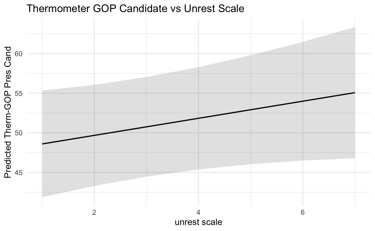
# plot_model from sjPlot package
plot_model(
  model  = full_model,
  type   = "pred",           # plot predicted value
  terms  = c("unrest_scale") # plot unrest_scale as predictor (x-axis)
) +
  theme_minimal() +
  ggtitle("Thermometer GOP Candidate vs Unrest Scale") +
  labs(y = "Predicted Therm-GOP Pres Cand")

Plot model with moderator term
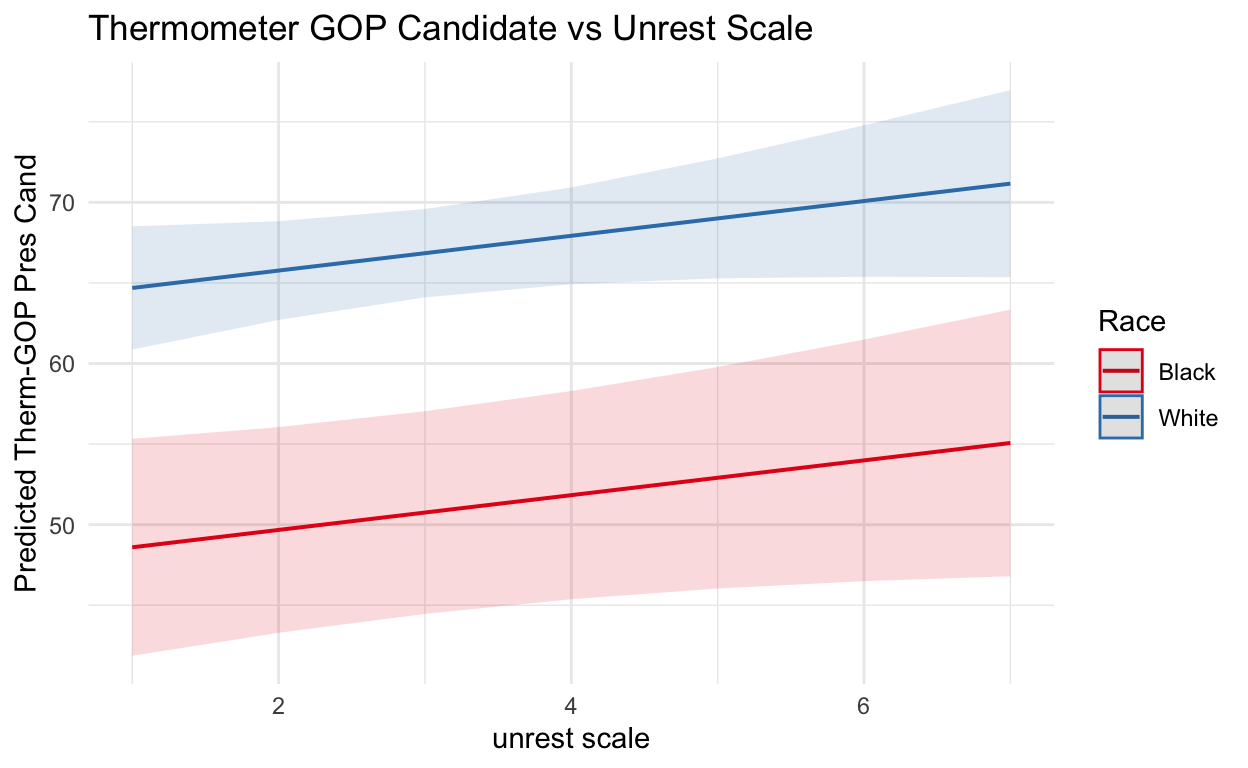
We can also look at how race moderates the main relationship. The slope of the relationship between the GOP Candidate Feeling Thermometer and the Urban Unrest Scale is the same for both groups (white and black) but whites, on average, feel more warmly towards the GOP candidate and blacks, on average, feel more cooly toward towards the GOP candidate (an intercept shift).
plot_model(
  model  = full_model,
  type   = "pred",                          # plot predicted value
  terms  = c("unrest_scale", "race_wb_fct") # plot unrest_scale as predictor
                                            # plot race_wb_fct as moderator
) +
  theme_minimal() +
  ggtitle("Thermometer GOP Candidate vs Unrest Scale") +
  labs(y     = "Predicted Therm-GOP Pres Cand",
       color = 'Race') # change legend title

This supplement was put together by Omar Wasow.