POL90: Statistics

Slides and Supplemental Materials for POL90

“Statistical thinking will one day be as necessary for efficient citizenship as the ability to read and write.”
— H.G. Wells

“We want facts. Factor, factor, factor is the motto which ought to stand at the head of all statistical work.”
— Florence Nightingale

“The sexy job in the next ten years will be statisticians… The ability to take data—to be able to understand it, to process it, to extract value from it, to visualize it, to communicate it—that’s going to be a hugely important skill.”
— Hal Varian, Chief Economist, Google,
McKinsey Insights, 1/2009

“For Today’s Graduate, Just One Word: Statistics”
— New York Times, 6/8/2009

“The best thing about being a statistician, is that you get to play in everyone’s backyard.”
— John Tukey,
New York Times, 7/28/2000

Course Description

In a world awash in data, how can we distinguish signals from noise? This course focuses on developing an intuition for statistics and applying it through data analysis, regression models and a final project. We will wrestle with what makes a good research question, play with data to see how statistical methods can help us make sense of real world concerns, and work at communicating quantitative findings clearly to broad audiences. Particular attention will be paid to applying these techniques in Junior Papers and Senior Theses. Coursework involves using the R statistical platform.

Overview

Broadly, the goal of this course is to develop your statistical literacy so that you can generate, interpret, convey and critique statistical findings. In particular, we will focus on developing an intuition for statistics, learning to apply statistical tools and practicing how to communicate meaningful statistical insights. Learning statistics is a lot like learning a language in that it requires lots of practice. Toward that end, the coursework emphasizes working with real data and developing skills that can be applied to your own research and future careers.

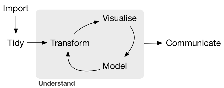
Throughout, we will focus on developing skills that allow one to move from working with messy, raw data to constructing appropriate models to communicating results clearly as illustrated in this diagram from R for Data Science by Grolemund and Wickham (2016).

Example: Survival in the Donner Party–An Observational Study

From Statistical Sleuth, Chapter 20 (p 602, 3e):

In 1846 the Donner and Reed families left Springfield, Illinois, for California by covered wagon. In July, the Donner Party, as it became known, reached Fort Bridger, Wyoming. There its leaders decided to attempt a new and untested route to the Sacramento Valley. Having reached its full size of 87 people and 20 wagons, the party was delayed by a difficult crossing of the Wasatch Range and again in the crossing of the desert west of the Great Salt Lake. The group became stranded in the eastern Sierra Nevada mountains when the region was hit by heavy snows in late October. By the time the last survivor was rescued on April 21, 1847, 40 of the 87 members had died from famine and exposure to extreme cold.

These data were used by an anthropologist to study the theory that females are better able to withstand harsh conditions than are males. (Data from D. K. Grayson, “Donner Party Deaths: A Demographic Assessment,” Journal of Anthropological Research 46 (1990): 223-42.)

For any given age, were the odds of survival greater for women than for men?

Code below from Supplement to Chapter 20 for POL90:

Importing and recoding data

# load data
donner <- Sleuth3::case2001 %>% 
  clean_names()

# view data
head(donner, 3)

  age    sex   status
1  23   Male     Died
2  40 Female Survived
3  40   Male Survived

# convert Survived/Died to ones/zeros
donner <- donner %>%
  mutate(
    # create numeric version of status
    survived = as.numeric(status == "Survived"),
    # make male = reference category
    sex = fct_relevel(sex, c("Male", "Female"))
    ) 

# view data
head(donner, 3)

  age    sex   status survived
1  23   Male     Died        0
2  40 Female Survived        1
3  40   Male Survived        1

Running and evaluating linear models

# run logistic regression with family = binomial
glm_sex <- glm(survived ~ sex,       family = binomial, data = donner)
glm_age <- glm(survived ~ age,       family = binomial, data = donner)
glm_sa  <- glm(survived ~ sex + age, family = binomial, data = donner)
glm_int <- glm(survived ~ sex * age, family = binomial, data = donner)

# print regression table
stargazer(
  glm_sex, glm_age, glm_sa, glm_int, 
  type = "html", 
  header = FALSE
  )

	Dependent variable:
	survived
	(1)	(2)	(3)	(4)
sexFemale	1.390**		1.600**	6.930**
	(0.671)		(0.755)	(3.400)
age		-0.066**	-0.078**	-0.032
		(0.032)	(0.037)	(0.035)
sexFemale:age				-0.162*
				(0.094)
Constant	-0.693*	1.820*	1.630	0.318
	(0.387)	(0.999)	(1.110)	(1.130)
Observations	45	45	45	45
Log Likelihood	-28.600	-28.100	-25.600	-23.700
Akaike Inf. Crit.	61.300	60.300	57.300	55.300
Note:	p<0.1; p<0.05; p<0.01

# assess trade-off between simplicity and explanatory power
anova(
    glm_sex, glm_sa, 
    test = "Chisq"
    ) %>%
  xtable() %>%
    print(
      type = "html",
      comment = FALSE # turn off message about package
         )

	Resid. Df	Resid. Dev	Df	Deviance	Pr(>Chi)
1	43	57.29
2	42	51.26	1	6.03	0.0141

# assess trade-off between simplicity and explanatory power
anova(
    glm_sa, glm_int, 
    test = "Chisq"
    ) %>%
  xtable() %>%
    print(
      type = "html",
      comment = FALSE # turn off message about package
         )

	Resid. Df	Resid. Dev	Df	Deviance	Pr(>Chi)
1	42	51.26
2	41	47.35	1	3.91	0.0480

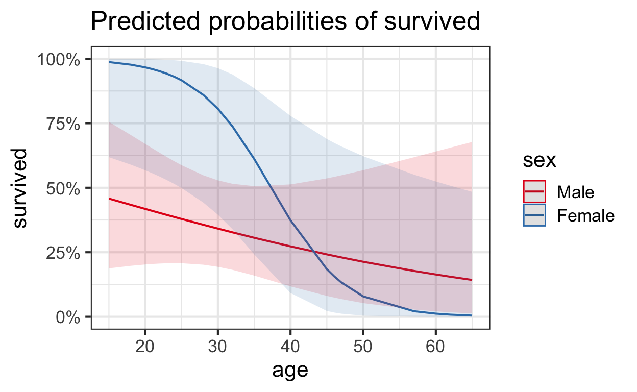
Visualize model

# plot model
sjPlot::plot_model(
    glm_int, 
    type = "pred", 
    terms = c("age [all]", "sex")
    ) 

Write-up statistical findings

While it generally appears that older adults were less likely than younger adults to survive, the data provide highly suggestive evidence that the age effect is more pronounced for females than for males (the two-sided p-value for interaction of gender and age is 0.05). Ignoring the interaction leads to an informal conclusion about the overall difference between men and women: The data provide highly suggestive evidence that the survival probability was higher for women (in the Donner Party) than for the men (two-sided p-value = 0.02 from a drop-in-deviance test). The odds of survival for women are estimated to be 5 times the odds of survival for similarly aged men (95% confidence interval: 1.2 times to 25.2 times, from a drop-in-deviance-based confidence interval).

Since the data are observational, the result cannot be used as proof that women were more apt to survive than men; the possibility of confounding variables cannot be excluded. Furthermore, since the 45 individuals were not drawn at random from any population, inference to a broader population is not justified.