This analysis uses data from the National Longitudinal Study of Adolescent to Adult Health (Add Health). Below is a brief overview of the data:
Add Health is a longitudinal study of a nationally representative sample of adolescents in grades 7-12 in the United States during the 1994-95 school year. The Add Health cohort has been followed into young adulthood with four in-home interviews, the most recent in 2008, when the sample was aged 24-32. Add Health combines longitudinal survey data on respondents’ social, economic, psychological and physical well-being with contextual data on the family, neighborhood, community, school, friendships, peer groups, and romantic relationships, providing unique opportunities to study how social environments and behaviors in adolescence are linked to health and achievement outcomes in young adulthood.
For more, see: https://www.icpsr.umich.edu/icpsrweb/DSDR/studies/21600
Load packages
library(kableExtra)
library(MASS)
library(janitor)
suppressMessages(library(stargazer))
suppressMessages(library(tidyverse))
library(naniar)

# fix randomization to get same results each time
set.seed(1234567)
Load data
To load data into R, the following commands may be helpful:
# verbose = TRUE tells us which the names of the data objects loaded
load("ICPSR_21600/DS0001/21600-0001-Data.rda", verbose = TRUE)
Loading objects:
  da21600.0001
# If you do not have the ICPSR_21600 data stored in the same folder as your
# your R Markdown file at the above path, you won't be able to knit code below
# assign data to shorter named file
ah1 <- da21600.0001
dim(ah1)
[1] 6504 2794names(ah1)[1:10]
 [1] "AID"     "IMONTH"  "IDAY"    "IYEAR"   "SCH_YR"  "BIO_SEX"
 [7] "VERSION" "SMP01"   "SMP03"   "H1GI1M"
# Example of loading a second data set:
load("ICPSR_21600/DS0028/21600-0028-Data.rda", verbose=TRUE)
Loading objects:
da21600.0028dim(da21600.0028)
[1] 5114 16names(da21600.0028)
 [1] "AID"      "CRP"      "CRP_FLAG" "EBV"      "EBV_FLAG" "C_CRP"
 [7] "C_SUBCLN" "C_INFECT" "CRP_MED1" "CRP_MED2" "CRP_MED3" "CRP_MED4"
[13] "CRP_MED5" "CRP_MED6" "CRP_MED7" "CRP_MED8"
ah28 <- da21600.0028
Recode, rename
You will also need to recode variables to account for issues like missing data (see the codebooks for how variables are coded). You may also want to rename variables for easier reference. For example,
ah1 <- ah1 %>%
  mutate(
    female = BIO_SEX == "(2) (2) Female",  # sex = female
    income = PA55,                         # parental income
    white  = H1GI6A == "(1) (1) Marked",   # race = white
    tv     = H1DA8,                        # hrs tv watched
    gamer  = H1DA10                        # hrs videogames played
  )

summary(ah1$tv)
   Min. 1st Qu.  Median    Mean 3rd Qu.    Max.    NA's
0.0 5.0 11.0 16.2 21.0 99.0 27 summary(ah1$gamer)
   Min. 1st Qu.  Median    Mean 3rd Qu.    Max.    NA's
0.0 0.0 1.0 2.9 3.0 99.0 12 summary(ah1$white)
   Mode   FALSE    TRUE    NA's
logical    2191    4294      19
Scrub
Remember, some variables are coded as numbers where you might want a categorical variable (and vice-versa). For example:
# look at levels of factor
levels(ah1$PA56)
[1] "(0) (0) No" "(1) (1) Yes"# use case_when to recode
ah1 <- ah1 %>%
mutate(
paybills = case_when(
PA56 == '(0) (0) No' ~ 0, # able to pay bills on time?
PA56 == '(1) (1) Yes' ~ 1,
TRUE ~ as.numeric(NA) # everything not assigned is NA
)
)
# check recoding worked
table(ah1$paybills)
   0    1
1009 4496
# Recode CLASSIFICATION OF HIGH SENSITIVITY C-REACTIVE PROTEIN (~stress)
levels(ah28$C_CRP)
[1] "(1) hsCRP < 1 mg/L - Low"       "(2) hsCRP 1 - 3 mg/L - Average"
[3] "(3) hsCRP > 3 mg/L - High"
ah28 <- ah28 %>%
mutate(
hscrp = case_when(
C_CRP == "(1) hsCRP < 1 mg/L - Low" ~ 1,
C_CRP == "(2) hsCRP 1 - 3 mg/L - Average" ~ 2,
C_CRP == "(3) hsCRP > 3 mg/L - High" ~ 3
)
)
summary(ah28$hscrp)
   Min. 1st Qu.  Median    Mean 3rd Qu.    Max.    NA's
      1       1       2       2       3       3     569
Workspace
The Add Health data sets can be very large. If, after loading,
merging, recoding, scrubbing and subsetting your data, you’d like to
remove large data.frames, the rm() command might be useful.
For example:
ah1_small <- ah1 %>%
  dplyr::select(AID, female, white, income, tv, gamer, paybills) %>% # subset data
  clean_names()

dim(ah1_small)
[1] 6504 7ah28 <- ah28 %>%
clean_names()
# remove original loaded data
rm(da21600.0001)
rm(da21600.0028)
# remove other larger data sets
rm(ah1)
Merging
The Add Health data consists of more than 30 separate files. Consequently, you will likely need to merge data from different data sets. For example,
[1] 5114 23ahnew[1:5,1:8] # look at 5 rows, 8 columns
       aid female white income tv gamer paybills   crp
1 57101310   TRUE FALSE     NA 33     0       NA 8.448
2 57103869  FALSE FALSE      9 24     7        1    NA
3 57109625  FALSE  TRUE      7 14     3        0 1.204
4 57111071  FALSE  TRUE     45 35     2        1 0.905
5 57113943  FALSE FALSE     12 10     4        1 5.363
Missingness
Now that we have a working data set, it is useful to view the
missingness in our data using the naniar package.
# load packages at top. Here, done in middle just for clarity
naniar::gg_miss_var(ahnew)
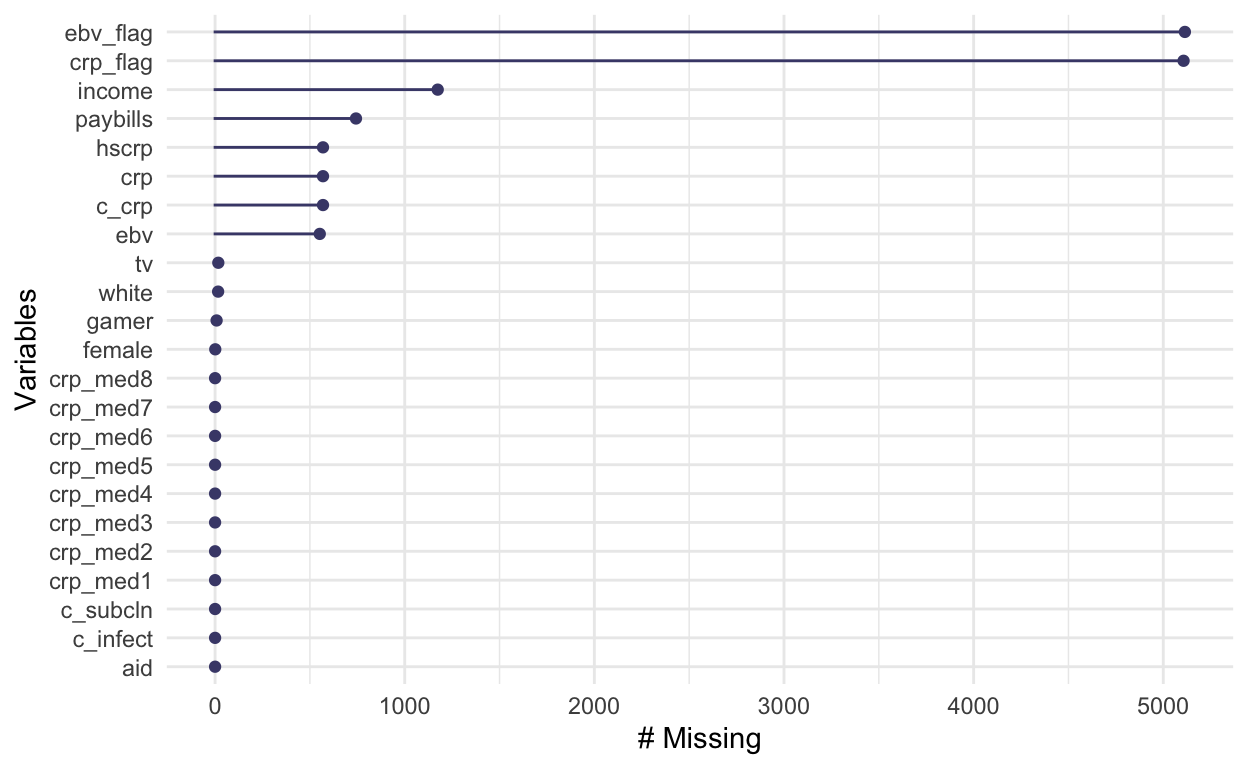
We have a lot of missingness in ebv_flag and
crp_flag but those are not important to the analysis that
follows and make it hard to see the scale of missingness in other
variables. So, let’s subset and look again:
# Look at missingness in subsetted data with essential vars
ah_subset <- ahnew %>%
  dplyr::select(aid, female, white, income, hscrp, tv, gamer, paybills)

gg_miss_var(ah_subset)
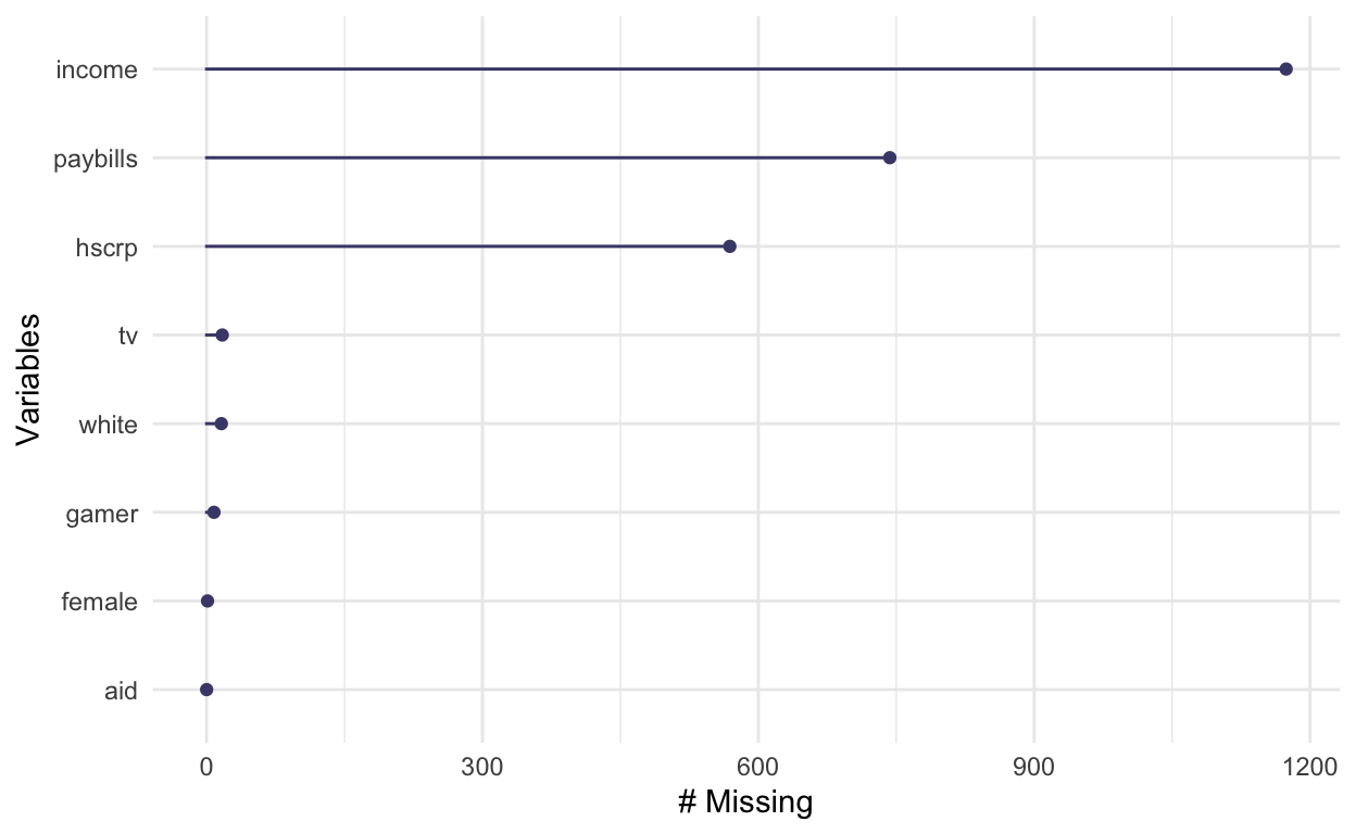
The income, paybills and hscrp
measures are important to our analysis and it would be useful to reduce
missingness through imputation rather than via listwise deletion. Also,
there is limited missingness in tv and
gamer.
Imputation with Amelia will work better if we provide
amelia a lot of detail about the variables. In particular,
consider:
idvars: what is the unique ID variable for observations? Or, are there other variables you don’t want imputed but you do want passed to the outputnoms: tell amelia this is an unordered factor, such as with asexorracemeasureords: tell amelia these are ordered factors (as in small, medium, large)bounds: a three column matrix to hold bounds on the imputations. Each row of the matrix should be of the form c(column.number, lower.bound, upper.bound)logs: any logged variables
# load packages at top. Here, done in middle just for clarity
library(Amelia)

# for demonstration, have some factor variables in data
ah_subset <- ah_subset %>%
  mutate(
    female = factor(female),
    white  = factor(white)
  )


# amelia cannot handle a newer type of data frame called a "tibble" or tbl_df
# just to be safe, makes sure you've got a plain old data.frame

ah_subset <- data.frame(ah_subset)


# identify columns that with bounds to include in bounds matrix option of amelia
match(c("income", "tv", "gamer"), names(ah_subset))
[1] 4 6 7# set up a matrix of bounds to pass to amelia
# matrix has three columns: 1st col = variable col #, 2nd = min, 3rd = max
bounds_matrix <- matrix( # tell amelia to bound some vars
ncol = 3, # 1st col = variable #, 2nd = min, 3rd = max
byrow = TRUE,
data = c(4, 0, 999, # bounds for col 4, income, 0 to 999
6, 0, 99, # bounds for col 6, tv hrs, 0 to 99
7, 0, 99) # bounds for col 7, gamer hrs, 0 to 99
)
ah_imputed <- amelia(
x = ah_subset, # data set
m = 1, # Number of imputations, typically 5, in pol90: 1
idvars = "aid", # what is the ID variable for observations
noms = c("female", "white"), # tell amelia these are unordered factors
ords = c("hscrp", "paybills"), # tell amelia these are ordered factors
bounds = bounds_matrix # tell amelia to bound some vars
)
-- Imputation 1 --

  1  2  3  4  5  6
The recommended approach for multiple imputation with Amelia is that researchers create five imputed data sets, each with slightly different imputed values for NAs, and run analyses on all five. As that is slightly beyond the scope of this class, we’ll just extract one imputation and continue the analysis on that.
# extract one imputed data set
ah_final <- ah_imputed$imputations$imp1
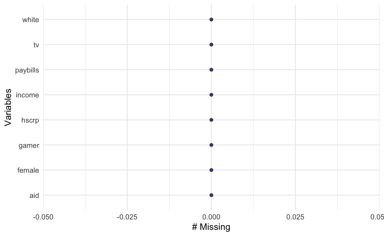
# check again for missingness
naniar::gg_miss_var(ah_final)
Saving
After recoding, scrubbing and merging your data, you may want to save the new data file so that you don’t have to repeat the earlier steps every time you run your analysis. For example:
# save new data to allow skipping earlier steps processing larger data
save(ah_final, file="ah_final.Rdata")

# Once you have saved a new data file, try eval=FALSE for earlier code chunks to
# skip scrubbing etc. and speed up compiling then just load the processed data before analysis.
# set eval=TRUE when loading orig data + scrubbing + recoding from scratch
# set eval=FALSE when skipping processing of data to load saved data frame
NOTE: You are encouraged to ask for help with any aspect of downloading, recoding, scrubbing, etc. stage of the analysis.
Analysis
Example plots and regressions with Add Health data.
# loading processed data saves compile time
#load("ah_final.Rdata", verbose=TRUE) # verbose reports what data loads
plot_gamer <- ah_final %>%
  ggplot() +
    aes(x = gamer,
        y = hscrp) +
    geom_point(alpha = .3) +
    geom_smooth(method = "lm") +
    theme_bw() +
    xlab("Hours Gaming") +
    ylab("Classification of hsCRP") # is gaming associated w/ more inflammation?


plot_tv <- ah_final %>%
  ggplot() +
    aes(x = tv,
        y = hscrp) +
    geom_point(alpha = .3) +
    geom_smooth(method = "lm") +
    theme_bw() +
    xlab("Hours TV") +
    ylab("Classification of hsCRP") # is gaming associated w/ more inflammation?

# comment out once cowplot is installed
# install.packages("cowplot", repos = 'http://cran.us.r-project.org')
suppressMessages(library(cowplot))
# see: https://cran.r-project.org/web/packages/cowplot/vignettes/introduction.html

cowplot::plot_grid(plot_gamer, plot_tv,
          labels = c("AUTO") ,
          ncol   = 2)
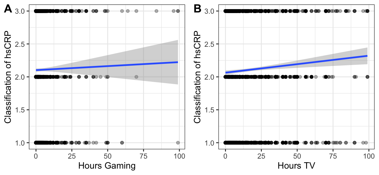
Figure 1: hsCRP vs gaming and TV use.
stargazer(
     lm1, lm2, lm3,
     dep.var.labels   = "Classification of hsCRP",
     covariate.labels = c("Hours Gaming", "Hours TV", "Can Pay Bills?",
                          "Female", "White", "Income"),
     title            = "OLS model of hsCRP vs gaming, tv and ability to pay bills",
     df               = FALSE,            # df option hides degrees of freedom to narrow cols
     header           = FALSE,        # hide package details
     table.placement  = "h", # try to place table here
     type             = 'html'
     )
| Dependent variable: | |||
| Classification of hsCRP | |||
| (1) | (2) | (3) | |
| Hours Gaming | 0.007*** | ||
| (0.002) | |||
| Hours TV | 0.003*** | ||
| (0.001) | |||
| Can Pay Bills? | -0.054* | ||
| (0.030) | |||
| Female | 0.355*** | 0.341*** | 0.335*** |
| (0.024) | (0.023) | (0.023) | |
| White | -0.047* | -0.038 | -0.047* |
| (0.025) | (0.025) | (0.025) | |
| Income | -0.001*** | -0.001*** | -0.001*** |
| (0.0002) | (0.0002) | (0.0002) | |
| Constant | 1.990*** | 1.960*** | 2.060*** |
| (0.027) | (0.031) | (0.033) | |
| Observations | 5,114 | 5,114 | 5,114 |
| R2 | 0.048 | 0.048 | 0.046 |
| Adjusted R2 | 0.048 | 0.048 | 0.046 |
| Residual Std. Error | 0.818 | 0.818 | 0.819 |
| F Statistic | 65.000*** | 64.800*** | 62.200*** |
| Note: | p<0.1; p<0.05; p<0.01 | ||
# logistic regression, dichotomizing y-variable
ah_final$hscrp_bin <- as.numeric(ah_final$hscrp==3)

lm4 <- glm(formula = hscrp_bin ~ gamer + female + white + income,
           data = ah_final, family = binomial)
lm5 <- glm(formula = hscrp_bin ~ tv + female + white + income,
           data = ah_final, family = binomial)

# we don't want 0,1 x var to be treated as continuous
ah_final$paybills_fct <- factor(ah_final$paybills)

lm6 <- glm(formula = hscrp_bin ~ paybills_fct + female + white + income,
           data = ah_final, family = binomial)
stargazer(
     lm4, lm5, lm6,
     dep.var.labels   = "Classification of hsCRP",
     covariate.labels = c("Hours Gaming", "Hours TV", "Can Pay Bills?",
                          "Female", "White", "Income"),
     title = "Logistic model of hsCRP vs gaming, tv and ability to pay bills",
     df = FALSE, # df option hides degrees of freedom stats to narrow columns
     header = FALSE, # hide package details
     table.placement = "h",
     type = 'html'
     )
| Dependent variable: | |||
| Classification of hsCRP | |||
| (1) | (2) | (3) | |
| Hours Gaming | 0.019*** | ||
| (0.005) | |||
| Hours TV | 0.006*** | ||
| (0.002) | |||
| Can Pay Bills? | -0.094 | ||
| (0.076) | |||
| Female | 0.947*** | 0.901*** | 0.887*** |
| (0.061) | (0.059) | (0.059) | |
| White | -0.139** | -0.122* | -0.145** |
| (0.063) | (0.063) | (0.063) | |
| Income | -0.003*** | -0.003*** | -0.003*** |
| (0.001) | (0.001) | (0.001) | |
| Constant | -0.700*** | -0.734*** | -0.538*** |
| (0.072) | (0.081) | (0.085) | |
| Observations | 5,114 | 5,114 | 5,114 |
| Log Likelihood | -3,321.000 | -3,325.000 | -3,329.000 |
| Akaike Inf. Crit. | 6,652.000 | 6,660.000 | 6,667.000 |
| Note: | p<0.1; p<0.05; p<0.01 | ||
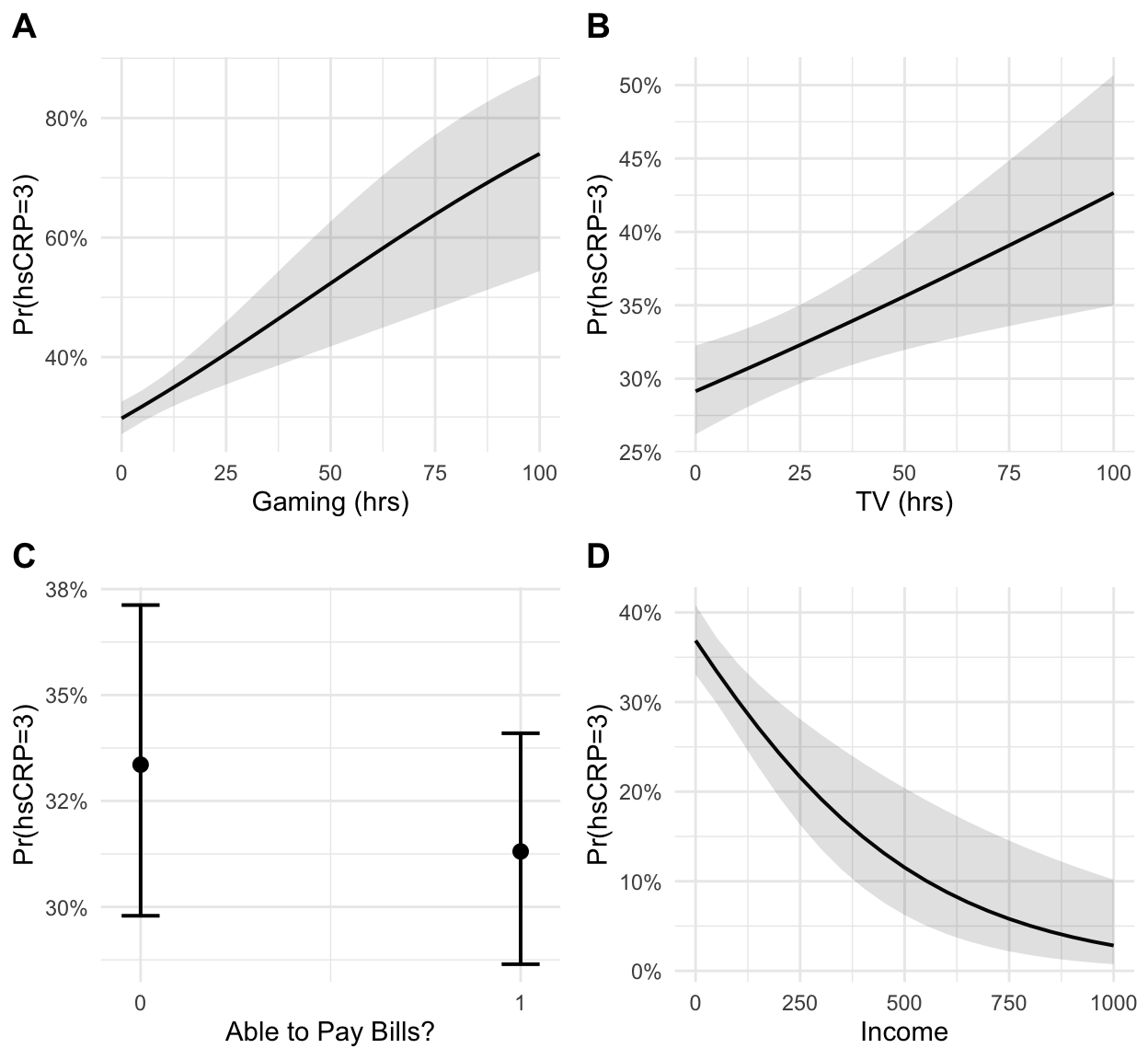
library(sjPlot)

# create sjPlot objects from models
plot_gamer  <- plot_model(lm4, type = "pred", terms = c("gamer"))
plot_tv     <- plot_model(lm5, type = "pred", terms = c("tv"))
plot_bills  <- plot_model(lm6, type = "eff",  terms = c("paybills_fct"))
plot_income <- plot_model(lm6, type = "pred", terms = c("income"))

# extract ggplot object from sjPlot object
# add labels to ggplot object
p1 <- plot_gamer +
    ggtitle("") +
    xlab("Gaming (hrs)") +
    ylab("Pr(hsCRP=3)")

p2 <- plot_tv +
    ggtitle("") +
    xlab("TV (hrs)") +
    ylab("Pr(hsCRP=3)")

p3 <- plot_bills +
    ggtitle("") +
    xlab("Able to Pay Bills?") +
    ylab("Pr(hsCRP=3)")

p4 <- plot_income +
    ggtitle("") +
    xlab("Income") +
    ylab("Pr(hsCRP=3)")


# plot ggplot objects in grid with labels
cowplot::plot_grid(
  p1, p2, p3, p4,
  ncol   = 2,
  labels = "AUTO"
  )
